Program Microsoft Excel 2007 - one of the two most popular programs in the package Microsoft Office... The most popular, of course, Microsoft Word ... Most recently most latest version the program was Excel 2003, but now there are 2007 and 2010 Excel. Consider how work in Excel 2007... This program is designed for drawing tables, presenting series of numbers in a visual form using diagrams and graphs. Also Microsoft program Excel It is used to carry out calculations and perform mathematical tasks of the most varied complexity: from simplifying routine mathematical operations to performing the most complex calculations. Most importantly, all this can be done quite simply, and no special knowledge is required.
Microsoft Excel works with files... Each file is a kind of book, consisting of sheets, where each sheet is a table. Various data can be entered into the cells of these tables: letters, designations, words, numbers. This data can be sorted, copied, moved. Also, other operations can be performed with data: textual, logical, mathematical ... Data can also be presented in a visual form - using graphs and diagrams.
Create an Excel file
Press the button Start in the lower left corner of the computer, select All programs, find Microsoft Office(if you have it installed), click on it, select Microsoft Office Excel, and run it with a double click.
After that, to create excel file, click on the big round button with squares in the upper left corner. In the window that appears, select Save as... The computer will open a new window with the contents of your computer, in which you will select the folder to save your file. In line File name where the default name is Book 1, put the cursor, and write a name for your future Excel file. You do not need to write the extension - it will be included in the name automatically. In the window below, where File type, leave Excel workbook.
While working on the file, save it periodically so that if your computer crashes or freezes, your work will not be lost. For subsequent saves, press the round button again, and select
Excel file structure. Sheets
Excel file- a kind of book that consists of sheets. You can switch between sheets by clicking on the corresponding sheet below, or on the arrows Forward and Back to the left of the sheet tabs (at the bottom of the working window of the program). There can be a lot of sheets in a book, they may not even be visible, and then you can switch between them exclusively using the arrows.
Each Excel sheet- a separate table. Using the icon to the right of the sheet tabs, you can insert new sheets. Sheets can also be renamed, deleted, moved. To do this, you either right-click on the sheet name. and select the desired operation in the window, or in the menu home select the items: Insert - Insert sheet, Delete - Delete sheet, Format - Rename sheet, Format - Move or copy sheet. You can also rearrange sheets by dragging the sheet tab to the right or left.
Now that you have learned how to create Excel files, consider working with tables and cells in this program.
More detailed information can be found in the sections "All courses" and "Usefulness", which can be accessed through the top menu of the site. In these sections, articles are grouped by topic into blocks containing the most detailed (as far as possible) information on various topics.
Sharing in Microsoft Excel allows multiple users to work with one file at once. Ten to twenty people on different computers simultaneously enter some data into one document. Where certain information is located, certain formulas work.
The "main user" has the ability to track the activities of the working group, add / remove members, edit conflicting changes. How to set up collaboration in Excel.
Features of working with a shared file
Not all tasks can be performed in a shared Excel workbook.
- Create Excel tables.
- Create, modify or view scripts.
- Delete sheets.
- Merge or split cells.
- Work with XML data (import, add, update, delete, etc.).
Exit: disable general access- perform a prohibited task - re-enable access.
Sharing limits a number of other tasks for participants:
| Unacceptable | Really |
| Insert or remove a group of cells | Add row or column |
| Add or change conditional formats | Work with existing formats |
| Turn on or modify the Data Validation tool | Work with existing scan settings |
| Create or edit charts, summary reports | Work with existing charts and pivot tables |
| Insert or edit pictures and graphics | View existing drawings and graphics |
| Insert or change hyperlinks | Follow existing hyperlinks |
| Assign, edit or delete passwords | Existing passwords are functional |
| Install or remove the protection of sheets and books | Existing protection works |
| Group, structure data; insert sublevels | Work with existing groups, structures and sublevels |
| Record, modify or view macros | Run existing macros that are not associated with unavailable tasks |
| Change or remove array formulas | Use existing formulas |
| Add new information to the data form | Search for information in the data form |
How to share an Excel file?
First, we decide which book we will "open" for editing by several participants at once. Create a new file and fill it with information. Or open an existing one.
- Go to the "Review" tab. Book Access Dialog Box.
- File access control - edit. We put a tick in front of "Allow several users to modify the file at the same time."
- Move on to the More Info tool to customize your multi-user editing options.
- Click OK. If we open public access to a new book, then we choose its title. If sharing is supposed for an existing file, click OK.
- Open the Microsoft Office menu. Select the "Save As" command. We select the format of the save file that will "go" on all user computers.
- Select the network resource / network folder that prospective contributors open. Click "Save".
Attention! You cannot use the web server to save the shared file.
- Data tab. "Connections".
- Change links / change links. If there is no such button, there are no associated files in the sheet.
- Go to the "Status" tab to check the existing connections. The OK button indicates that the links are working.
Opening a shared workbook
- Open the Microsoft Office menu.
- Click "Open".
- Choosing a shared book.
- When the book is open, click on the Microsoft Office button. Go to the Excel Options tab (at the bottom of the menu).
- "Are common" - " Personal customization" - "Username". Enter identification information (name, nickname).
Everything. You can edit information, enter new ones. Save after work.
Occasionally, when you open a file-sharing Excel workbook, a "File Locked" entry appears. Can't save. When you open it again, it turns out that sharing is disabled. Possible reasons Problems:
- Several users edit the same part of the document. For example, they drive different data into one cell. A blocking occurs.
- While using a shared file, a change log is kept (who logged in, when, what did). The book enlarges. Begins to "glitch".
- Someone from the users was deleted, but they haven’t been told about it yet. Then the lock can appear only on his computer.
What you can do if file sharing is blocked:
- Clear or delete the change log.
- Clean the contents of the file.
- Cancel and then reactivate sharing.
- Open xls workbook in OpenOffice. And save it to xls again.
It is noticed that the entry "File locked" appears less often in newest versions Excel.
How to delete a user
- On the "Review" tab, open the "Book Access" menu.
- In the "Edit" section, we see a list of users.
- Choose a name - click "Delete".
Make sure users are finished with the file before deleting.
How to turn off sharing mode in Excel
- Review Tab - Changes - Highlight Changes.
- We set the parameters of the "Fixes". By time - "everything". The checkboxes opposite "By user" and "In range" are unchecked. On the contrary, “make changes to separate sheet" - costs. Click OK.
- The Changelog will open. It can be saved either.
To turn off sharing to Excel file, on the "Review" tab, click "Book access" and uncheck the box next to "Allow multiple users to modify the file".
Only one user should remain on the list - you.
Hello friends. Today I will tell you how to create an Excel file, open an existing one, save it and close it.
Every worker Excel workbook stored in a separate file. Therefore, it is very important to be able to handle files correctly. Here I will describe several ways to perform actions with documents. I advise you to try each one and choose which one is the most convenient, or maybe you will use many of them.
All calculations on this blog are from Microsoft Office 2013. If you are using a different version, some commands and windows may look slightly different, but their general meaning remains the same. If you did not find the described toolkit in your version of the program - ask in the comments or through the form feedback... I will definitely answer your questions.
Create an Excel document
If you don't have Excel open yet, click on the MS Excel shortcut on the desktop or in the menu Start... After loading Excel, a start window with a choice of templates will appear. To create a new document, click on one of them, or select Blank Book.
 Excel start window
If MS Excel is already running, for creating:
- Press the key combination Ctrl + N. After clicking, a new workbook will be created immediately
- Execute the tape command File - New. Its execution will lead to the opening of the start window, where you can create a file from a template, or a blank book.
How to open an Excel document
If Excel is not running yet to open the generated file, find it in Windows Explorer and double-click on it with the mouse. MS Excel will be launched and the document of your choice will open immediately.
If the program is already running There are several ways to open a workbook:

If you select the location Computer - Browse in the Open window, an explorer window will open, where you can select a filter for the file to open, as well as a way to open it:
- Open- opens the selected Excel file for editing
- Open for reading- opens the file without the possibility of editing
- Open as copy- creates a duplicate of the document and opens it with the ability to edit
- Open in browser- if this option is supported, opens the workbook in an Internet browser
- Open in Protected View- opens the document using Protected View
- Open and restore- the program will try to restore and open a file that was abnormally closed without saving
Opening a file from disk
Saving an Excel document
While Microsoft Excel has good autosave and data recovery tools, I recommend getting in the habit of saving your workbook from time to time, even if you're not finished with it. At the very least, you will feel more confident that the results of your work will not be lost.
- Use the keyboard shortcut Ctrl + S
- Use the key combination Shift + F12, or F12 (to save the document under a new name)
- Click Save on the Quick Access Toolbar
- Run the ribbon command File - Save, or File - Save As (if you want to save the book as a new document)
If this is your first time saving your workbook, either of these commands will open the Save As window, where you can select the save location, file type, and file name. To do this, click the Browse button.
If you have saved the document before, the program will simply save the file over the last saved version.
How to close an Excel workbook
When you're done with the file, it's best to close it to free up system memory. You can do it in the following ways:
- Click on the cross(x) in the upper right corner of the program window
- Execute command File - Close
- Double click on the pictogram system menu in the upper left corner of the window
Excel system menu icon - Use the keyboard shortcuts Ctrl + W, or Alt + F4
If at the time of closing the file contains unsaved changes, the program will ask what to do:
- Save- save all changes and close the document
- Do not save- close the workbook without saving
- Cancellation- do not close the file
Close Excel workbook
That's all the ways to handle Excel files. And in the next post I'll show you how to set up autosave for your workbook. See you!
In the first material Excel 2010 for beginners, we will get acquainted with the basics of this application and its interface, learn how to create spreadsheets, as well as enter, edit and format data in them.
Table of contents
- Introduction
- Interface and control
- Data entry and editing
- Formatting data
- Cell data format
- Conclusion
Introduction
I think I will not be mistaken if I say that the most popular application included in the Microsoft Office package is the Word test editor (processor). However, there is another program that any office worker rarely does without. Microsoft Excel (Excel) refers to software products which are called spreadsheets. WITH using Excel, in a visual form, you can calculate and automate the calculations of almost anything, from a personal monthly budget to complex mathematical and economic-statistical calculations containing large amounts of data sets.
One of key features spreadsheets is the ability to automatically recalculate the value of any desired cells when the content of one of them changes. To visualize the obtained data, based on groups of cells, you can create various types of charts, pivot tables and maps. At the same time, spreadsheets created in Excel can be inserted into other documents, as well as saved in a separate file for later use or editing.
To call Excel simply a “spreadsheet” would be somewhat incorrect, since this program has enormous capabilities, and in terms of its functionality and range of tasks, this application, perhaps, can even surpass Word. That is why, within the framework of the series of materials "Excel for Beginners", we will get acquainted only with the key features of this program.
Now, after the end of the introductory part, it's time to get down to business. In the first part of the cycle, for better assimilation of the material, as an example, we will create a regular table that reflects personal budgetary expenses for six months like this:
But before starting to create it, let's first look at the basic elements of the interface and controls of Excel, as well as talk about some of the basic concepts of this program.
Interface and control
If you are already familiar with Word editor, then it will not be difficult to understand the Excel interface. After all, it is based on the same ribbon, but only with a different set of tabs, groups and commands. At the same time, in order to expand the work area, some groups of tabs are displayed only if necessary. You can also minimize the ribbon altogether by double-clicking on the active tab with the left mouse button or by pressing the Ctrl + F1 key combination. Returning it to the screen is done in the same way.
It is worth noting that in Excel for the same command, there can be several ways to call it at once: through the ribbon, from the context menu, or using a combination of hot keys. Knowledge and use of the latter can greatly speed up the work in the program.
The context menu is context sensitive, that is, its content depends on what the user is doing at the moment. The context menu is invoked by right-clicking on almost any object in MS Excel. This saves time because it displays the most frequently used commands for the selected object.
Despite such a variety of controls, the developers went further and provided users in Excel 2010 with the ability to make changes to the built-in tabs and even create their own with those groups and commands that are used most often. To do this, right-click on any tab and select the item Customizing the Ribbon.
In the window that opens, in the menu on the right, select the desired tab and click on the button Create a tab or To create a group, and in the left menu the desired command, then click the button Add... In the same window, you can rename existing tabs and delete them. To cancel erroneous actions, there is a button Reset, which returns the tab settings to their initial settings.
Also, the most frequently used commands can be added to Quick Access Toolbar located in the upper left corner of the program window.
This can be done by clicking on the button Customizing the Quick Access Toolbar, where it is enough to select the required command from the list, and if the required command is absent in it, click on the item Other commands.
Data entry and editing
Files created in Excel are called workbooks and have the extension "xls" or "xlsx". In turn, a workbook consists of several worksheets. Each worksheet is a separate spreadsheet that can be interconnected if necessary. The active workbook is the one you are currently working with, for example, into which you enter data.
After starting the application, a new book named "Book1" is automatically created. By default, a workbook consists of three worksheets named “Sheet1” to “Sheet3”.
The working area of the Excel worksheet is divided into many rectangular cells. Horizontally merged cells are rows, and vertically merged columns. To be able to explore a large amount of data, each worksheet of the program has 1,048,576 lines numbered with numbers and 16,384 columns designated with letters of the Latin alphabet.
Thus, each cell is the intersection of various columns and rows on the sheet, forming its own unique address, consisting of the letter of the column and the row number to which it belongs. For example, the name of the first cell is A1 because it is at the intersection of column "A" and row "1".
If the app includes Formula bar which is located immediately below Ribbon, then to the left of it is Name field where the name of the current cell is displayed. Here you can always enter the name of the cell you are looking for, to quickly jump to it. This feature is especially useful on large documents with thousands of rows and columns.
Also for viewing different areas of the sheet, scroll bars are located at the bottom and on the right. In addition, you can use the arrow keys to navigate the Excel workspace.
To start entering data in the desired cell, you must select it. To go to the desired cell, left-click on it, after which it will be surrounded by a black frame, the so-called indicator of the active cell. Now just start typing on the keyboard, and all the information you enter will appear in the selected cell.
When entering data into a cell, you can also use the formula bar. To do this, select the required cell, and then click on the field of the formula bar and start typing. In this case, the information entered will be automatically displayed in the selected cell.
After finishing data entry press:
- Press "Enter" - the next active cell will be the cell below.
- Key "Tab" - the next active cell will be the cell to the right.
- Click on any other cell and it will become active.
To change or delete the contents of any cell, double-click on it with the left mouse button. Move the flashing cursor to the desired location to make the necessary edits. As with many other applications, the arrow keys, Del, and Backspace are used to delete and make corrections. If desired, all necessary edits can be made in the formula bar.
The amount of data that you will enter into a cell is not limited to its visible part. That is, the cells of the working area of the program can contain both one number and several paragraphs of text. Each Excel cell can accommodate up to 32,767 numeric or text characters.
Formatting cell data
After entering the names of the rows and columns, we get a table of the following type:
As you can see from our example, several names of expense items "went" beyond the boundaries of the cell, and if the adjacent cell (cells) also contain some information, then the entered text partially overlaps with it and becomes invisible. And the table itself looks rather ugly and unpresentable. At the same time, if you print such a document, then the current situation will remain - it will be quite difficult to disassemble in such a table what is going to be quite difficult, as you can see for yourself from the picture below.
To make a spreadsheet document neater and more beautiful, you often have to change the size of rows and columns, the font of the cell content, its background, align the text, add borders, and so on.
First, let's tidy up the left column. Move the mouse cursor over the border of columns "A" and "B" in the row where their names are displayed. When you change the mouse cursor to a characteristic symbol with two oppositely directed arrows, press and hold left key, drag the dotted line that appears in the desired direction to expand the column until all the titles fit within one cell.
You can do the same with a string. This is one of the easiest ways to resize the height and width of the cells.
If you need to set the exact sizes of rows and columns, then on the tab home in Group Cells select item Format... In the menu that opens using the commands Line height and Column width you can set these parameters manually.
Very often it is necessary to change the parameters of several cells and even an entire column or row. In order to select an entire column or row, click on its name above or on its number on the left, respectively.
To select a group of adjacent cells, stroke them with the cursor, hold left button mice. If it is necessary to select the scattered fields of the table, then press and hold the "Ctrl" key, and then click on the required cells.
Now that you know how to select and format multiple cells at once, let's center the month names in our table. Various commands for aligning content inside cells are located on the tab home in a group with a telling name Alignment... Moreover, for a table cell, this action can be performed both relative to the horizontal direction and vertical.
Circle the cells with the name of the months in the header of the table and click the button Align Center.
In Group Font in the tab home you can change the font type, size, color and style: bold, italic, underlined, and so on. There are also buttons for changing the borders of a cell and its fill color. All these functions will be useful for us to further change the appearance of the table.
So, first, let's increase the font of the column and column names of our table to 12 points, and also make it bold.
Now, first select the top row of the table and set it to a black background, and then in the left column, cells A2 to A6, dark blue. This can be done using the button Fill color.
You've probably noticed that the color of the text in the top row has merged with the background color, and the names in the left column are poorly readable. Let's fix this by changing the font color using the button Text color to white.
Also using the already familiar command Fill color we have given the background of odd and even rows with numbers a different blue tint.
To prevent the cells from merging, let's define borders for them. Determination of borders occurs only for the selected area of the document, and can be done both for one cell and for the entire table. In our case, select the entire table, then click on the arrow next to the button Other boundaries everyone in the same group Font.
The menu that opens displays a list of quick commands, with which you can choose to display the desired boundaries of the selected area: bottom, top, left, right, outer, all, and so on. It also contains commands for drawing borders by hand. At the very bottom of the list is the item Other boundaries which allows you to specify in more detail the necessary parameters of the borders of the cells, which we will use.
In the window that opens, first select the type of border line (in our case, a thin solid), then its color (choose white, since the background of the table is dark) and finally, those borders that should be displayed (we chose the inner ones).
As a result, using a set of commands of just one group Font we transformed ugly appearance tables into quite presentable, and now knowing how they work, you yourself will be able to come up with your own unique styles for the design of spreadsheets.
Cell data format
Now, in order to complete our table, it is necessary to properly format the data that we enter there. Recall that in our case these are cash costs.
To each of the cells spreadsheet you can enter different types data: text, numbers and even graphics. That is why in Excel there is such a thing as "cell data format", which serves to correctly process the information you enter.
Initially, all cells have General format allowing them to contain both text and digital data. But you are free to change this and choose: numeric, monetary, financial, percentage, fractional, exponential, and formats. In addition, there are formats for date, time of postal codes, telephone numbers and personnel numbers.
For the cells of our table containing the names of its rows and columns, the general format (which is set by default) is quite suitable, since they contain text data. But for the cells in which budget expenditures are entered, the monetary format is more suitable.
Select cells in the table containing information on monthly expenses. On the ribbon in the tab home in Group Number click the arrow next to the field Number Format, after which a menu will open with a list of the main available formats. You can select the item Monetary right here, but we will select the very bottom line for a more complete overview Other number formats.
In the window that opens, in the left column, the name of all number formats, including additional ones, will be displayed, and in the center, various settings for their display.
Having selected the currency format, at the top of the window you can see how the value in the table cells will look like. Slightly below mono set the number of displaying decimal places. So that the pennies do not clutter up the table fields, we will set the value here equal to zero. Next, you can select the currency and display negative numbers.
Now our sample table is finally complete:
By the way, all the manipulations that we did with the table above, that is, the formatting of cells and their data can be performed using the context menu by right-clicking on the selected area and selecting the item Cell format... In the window of the same name, for all the operations we have considered, there are tabs: Number, Alignment, Font, The border and Fill.
Now, after finishing work in the program, you can save or the result obtained. All these commands are in the tab File.
Conclusion
Probably, many of you will ask the question: "Why create such tables in Excel, when all the same can be done in Word, using ready-made templates?" That is how it is, only to perform all sorts of mathematical operations on cells in text editor impossible. You almost always enter the information in the cells yourself, and the table is only a visual representation of the data. And it is not very convenient to make voluminous tables in Word.
In Excel, the opposite is true, tables can be arbitrarily large, and the value of cells can be entered either manually or automatically calculated using formulas. That is, here the table acts not only as a visual aid, but also as a powerful computational and analytical tool. Moreover, cells can be interconnected with each other not only within one table, but also contain values obtained from other tables located on different sheets and even in different books.
You will learn how to make a table "smart" in the next part, in which we will get acquainted with the basic computational capabilities of Excel, the rules for constructing mathematical formulas, functions and much more.
You can use Object Linking and Embedding (OLE) to include content from other programs, such as Word or Excel.
OLE is supported by many different programs, and OLE is used to create content that is created in one program and available in another program. For example, you can insert an Office Word document into an Office Excel workbook. To see what types of content you can insert in the group text in the tab Insert press the button an object... In field Object type only programs installed on your computer that support OLE objects are displayed.
General information about related and embedded objects
When copying data between Excel or any program that supports OLE technology such as Word, you can copy this data as related object or an embedded object. The main differences between linked and embedded objects are in where the data is stored, as well as how the object will be updated after you put it in the target file. Embedded objects are stored in the workbook in which they are inserted and are not updated. Linked objects are saved as separate files and can be updated.
Linked and embedded objects in a document
1. the embedded object has no connection to the original file.
2. the linked object is linked to the original file.
3. the source file updates the linked object.
When to use linked objects
If you want the information in the target file to update when the data in the source file changes, use linked objects.
When using a linked object, the original data is retained in the original file. The resulting file displays a view of related data that contains only the original data (and the size of the object if the object is an Excel chart). The source file must be available on your computer or on the network to keep in touch with the original data.
Linked data can be updated automatically when the original data in the source file changes. For example, if you select a paragraph in Word document and then insert it as a linked object into an Excel workbook, then when the data in the Word document changes, you can update the data in Excel.
Using embedded objects
If you don't want the copied data to be updated when the source file changes, use an embedded object. The source code version is fully embedded in the book. If you copy data as an embedded object, the destination file requires more disk space than when binding the data.
When a user opens a file on another computer, they can view the embedded object without accessing the original data. Because the embedded object has no links to the original file, the object is not updated when the original data changes. To modify an embedded object, double-click the object to open it and modify it in the original program. The original program (or another program that supports object editing) must be installed on your computer.
Change how an OLE object is displayed
You can display a linked object or an embedded object in a workbook as it appears in the source program or as an icon. If the book will be viewed on the Internet and you do not plan to print the book, you can display the object as an icon. This reduces the amount of displayed space the object takes up. Double-click the icon to view where you want to display information.
Embedding an object on a sheet
Insert a link to a file
Note:
Creating an object in Excel

Embedding an object on a sheet

Insert a link to a file
Sometimes you just need to add a reference to the object, not embed it. You can do this if the workbook and the object you want to add are stored on a SharePoint site, shared network drive, or similar permanent location. This is useful if the linked object changes, as the link will always open its latest version.
Note: If you move the linked file, the link will not work.
Creating an object in Excel
You can create an object using another program without leaving the book. For example, if you want to add more detailed description to a chart or table, you can create an embedded document in Excel, such as Word or PowerPoint. You can insert an object directly into a sheet, or add an icon to open a file.
Linking and Embedding Content from Another Program Using OLE
You can link or embed content or a piece of content from another program.

Embedding content from another program
Linking or embedding partial content from another program

Change how an OLE object is displayed
To display the content, uncheck the box Show as icon .
To display the icon, check the box in as an icon... Alternatively, you can change the default icon image or label. To do this, press the button Change Icon, and then select the desired icon from the list badges or enter a label in the field heading .
an objectObject type(For example, Document object) and select the command transform.
Managing updates to related objects
You can customize links to other programs so that they are updated in the following ways: automatically when you open the destination file; manually if you want to view previous data before updating with new data from the original file; or, if you are requesting an update, whether automatic or manual updates are enabled.
Installing an update manually linking to another program

Configuring automatic link updates to another program
Issues: unable to update automatic links in worksheet
Parameter automatically can be overridden with the command update links in other documents Excel.
To provide automatic update automatic links to OLE objects:
Updating a link to another program
Editing content from an OLE program
In Excel, you can change content that is linked or embedded from another program.
Modifying a linked object in the original program
Modifying an embedded object in a source program
Double-click an embedded object to open it.
Make the necessary changes to the object.
If you are editing an object in place in open program, click anywhere outside the object to return to the destination file.
If you are modifying the embedded object in the source program in a separate window, exit the source program to return to the destination file.
Note: When you double-click on some embedded objects, for example video and audio clips, the object is played instead of opening the program. To change one of these embedded objects, right-click the icon or object, select an objectObject type(For example, object clip media) and press the button change.
Modifying an embedded object in a program other than the original
To convert the embedded object to the type specified in the list, click convert to.
To open the embedded object as the type that you specified in the list without changing the type of the embedded object, click activate.
Select the embedded object that you want to modify.
Right-click an icon or object, hover over an objectObject type(For example, Document object) and select the command transform.
Perform one of the following actions.
Selecting an OLE Object Using the Keyboard
Press CTRL + G to open a dialog box Go to .
Click the button highlight, select item objects and then click OK.
Press the Tab key until you select the item you want.
Press SHIFT + F10.
Move the pointer over an item, or diagram and select the command change.
Q: when I double click on a linked or embedded object, I get a "cannot be modified" message
This message appears if the source file or source program cannot be opened.
Make sure the original program is available If the original program is not installed on your computer, convert the object to the file format installed for the program.
Make sure the memory fits Make sure you have enough memory to run the original program. Close other programs if necessary to free up memory.
Close all dialog boxes If the original program is running, make sure there are no open dialog boxes. Switch to the original program and close all open dialog boxes.
Closing the source file If the source file is a linked object, make sure that it is not open by another user.
Make sure the name of the original file has not changed If the original file you want to change is linked, make sure it has the same name as when you created the link and that it has not been moved. Select the linked object and then in the group " connections"on the tab" data"click command" change links"to see the name of the original file. If the original file has been renamed or moved, use the button change source in the dialog box changing ties to find the original file and re-link the link.
additional information
You can always ask the Excel Tech Community a question, ask for help in the Answers community, and also suggest new function or improvement on the website
Today everyone seems to be moving to cloud storage, so why are we worse? New technologies for sharing Excel data over the Internet is a simple method that provides many opportunities and benefits that you can use.
With the advent of Excel Online, you no longer need cumbersome HTML code to place spreadsheets on the Internet. Simply save your workbook online and access it literally from anywhere, share it with others, and work together on the same spreadsheet. Using Excel Online, you can insert an Excel sheet into a website or blog and let your visitors interact with it to get exactly the information they want to find.
How to send Excel 2013 worksheets online
Everything Excel sheets Online are stored in the OneDrive web service ( former SkyDrive). As you probably know, this online storage appeared some time ago, and now it is integrated into Microsoft Excel as a one-click interface command. In addition, guests, i.e. other users with whom you share your spreadsheets no longer need their own Microsoft account in order to view and edit those Excel files that you have shared with them.
If you still do not have account OneDrive, you can create one right now. This service is simple, free and definitely deserves your attention, since most of the applications in the Microsoft Office 2013 suite (not only Excel) support OneDrive. After registration, follow these steps:
1. Log in to your Microsoft account
Make sure you are signed in to your Microsoft account from Excel 2013. Open an Excel workbook and look at its right top corner... If you see your name and photo there, then go to the next step, otherwise click Sign in(Entrance).
Excel will display a window asking you to confirm that you really want to let Office connect to the Internet. Click on Yes(Yes) and then enter your account details Windows entries Live.
2. Save your Excel sheet to the cloud
Make sure, for your own peace of mind, that the workbook you need is open, that is, the one that you want to share on the Internet. I want to share a book Holiday Gift List so that my family and my friends can watch it and contribute

With the workbook you want to open, go to the tab File(File) and click Share(Share) on the left side of the window. By default, the option will be selected. Invite People(Invite other people), then you need to click Save to cloud(Save to Cloud) on the right side of the window.

After that, choose a location to save the Excel file. First in the list on the left is OneDrive, and it's selected by default. You just need to specify the folder to save the file on the right side of the window.
Comment: If you do not see the OneDrive menu item, then you do not have a OneDrive account, or you are not signed in to your account.

I have already created special folder Gift Planner and it is shown in the list of recent folders. You can select any other folder by clicking the button Browse(Review) below area Recent Folders(Recent folders), or create new folder by right-clicking and choosing from the context menu New(Create)> Folder(Folder). When the desired folder is selected, press Save(Save).
3. We provide general access to an Excel sheet saved on the Internet
Your Excel workbook is already online and you can view it on your OneDrive. If you need to open shared access to Excel sheets saved on the Internet, then you just have to take one step - choose one of the methods of sharing offered by Excel 2013:

Advice: If you want to limit the area of the Excel workbook that is available for viewing by other users, open the tab File(File) section Info(Details) and press Browser View Options(Browser View Options). Here you can customize which sheets and which named items can be displayed on the Internet.
That's all! Your Excel 2013 workbook is now online and can be accessed by selected users. And even if you do not like to work with someone, this method will allow you to access Excel files from anywhere, no matter if you are in the office, working from home or traveling somewhere.
Working with workbooks in Excel Online
If you are a confident inhabitant of the Cloudy Universe, then master Excel Online without any problems during your lunch break.
How to create a workbook in Excel Online
To create a new book, click the small arrow next to the button Create(Create) and in the drop-down list select Excel workbook(Excel workbook).

To rename your online book, click the default name and enter a new one.

To upload an existing workbook to Excel Online, click Upload(Download) in the OneDrive toolbar and specify desired file saved on the computer.

How to edit workbooks in Excel Online
After you have opened a workbook in Excel Online, you can work with it using Excel Web App (just like with Excel installed on personal computer), i.e. enter data, sort and filter, calculate using formulas, and visualize data using charts.
There is only one significant difference between the web version and the local version. Excel version... Excel Online doesn't have a button Save(Save) because it saves the workbook automatically. If you change your mind, click Ctrl + Z to undo the action, and Ctrl + Y to redo the undone action. For the same purpose, you can use the buttons Undo(Cancel) / Redo(Revert) tab Home(Home) section Undo(Cancel).
If you try to edit some data, but nothing happens, then most likely the book is open in read-only mode. To enable editing mode, click Edit workbook(Edit book)> Edit in Excel Web App(Edit in Excel Online) and make quick changes right in your web browser. To access more advanced data analysis capabilities such as pivot tables, sparklines, or linking to external source data, click Edit in Excel(Open in Excel) to switch to Microsoft Excel on your computer.

When you save the sheet in Excel, it will be saved where you originally created it, that is, in cloud storage OneDrive.
Advice: If you want to make quick changes in several books, then the best way is to open the list of files in your OneDrive, find the book you need, right-click on it and select the required action from the context menu.

How to share your worksheet with others in Excel Online

... and then choose one of the options:
- Invite People(Send link to access) - and enter the address Email people you want to give access to the book.
- Get a link(Get link) - and put this link in email, post on the website or social networks.
You can also set access rights for contacts: the right to view only or give permission to edit the document.

When several people are editing a worksheet at the same time, Excel Online immediately shows their presence and the updates made, provided that everyone is editing the document in Excel Online, and not in local Excel on the computer. If you click the small arrow next to the person's name in the upper right corner of the Excel sheet, you can see which cell that person is currently editing.

How to block editing of specific cells on a shared worksheet
If you are sharing online sheets with your team, you might want to give them edit rights to only certain cells, rows, or columns of an Excel document. To do this, in Excel on your local computer, you need to select the range (s) that you allow to edit, and then protect the sheet.

How to embed an Excel worksheet in a website or blog

Comment: The embed code is an iframe, so make sure your site supports this tag and your blog allows it to be used in posts.
Embedded Excel Web App
What you see below is an interactive Excel sheet that demonstrates this technique in action. This table calculates how many days are left until your next birthday, anniversary, or some other event, and colors the gaps in different shades of green, yellow, and red. In Excel Web App, you just need to enter your events in the first column, then try changing the corresponding dates and see the results.
If you are curious about the formula used here, then please see the article How to set up conditional date formatting in Excel.
Translator's note: In some browsers, this iframe may display incorrectly or not display at all.
Mashups in Excel Web App
If you want to create a closer interaction between your Excel web sheets and other web applications or services, you can use the JavaScript API available on OneDrive to create interactive mashups from your data.
Below is the Destination Explorer mashup created by the Excel Web App team as an example of what developers can create for your website or blog. This mashup uses the Excel Services JavaScript API and Bing Maps to help site visitors navigate their journey. You can choose a place on the map, and the mashup will show you the weather in this place or the number of tourists visiting these places. The screenshot below shows our location
Microsoft Excel is convenient for compiling tables and making calculations. The work area is a set of cells that you can fill with data. Subsequently - to format, use for building graphs, charts, summary reports.
Working with Excel spreadsheets for novice users may seem daunting at first glance. It differs significantly from the principles of constructing tables in Word. But we'll start small: by creating and formatting the table. And at the end of the article, you will already understand that best tool for creating tables than Excel can be imagined.
How to create a spreadsheet in Excel for dummies
Working with spreadsheets in Excel for dummies takes no rush. You can create a table different ways and for specific purposes, each method has its own advantages. Therefore, first we will visually assess the situation.
Take a close look at the spreadsheet worksheet:
It is a lot of cells in columns and rows. Essentially a table. The columns are designated in Latin letters. Lines - in numbers. If we print this sheet, we get a blank page. Without any boundaries.
First, let's learn how to work with cells, rows and columns.
How to highlight a column and row
To select the entire column, click on its name (Latin letter) with the left mouse button.

To select a line - by line name (by number).

To select several columns or rows, left-click on the name, hold and drag.
To select a column using hot keys, place the cursor in any cell of the desired column - press Ctrl + Space. To select a line - Shift + space.
How to change cell borders
If the information does not fit when filling the table, you need to change the borders of the cells:


To change the width of the columns and the height of the rows at once in a certain range, select an area, increase 1 column / row (move it manually) - the size of all selected columns and rows will automatically change.

Note. To return to the previous size, you can click the Cancel button or the keyboard shortcut CTRL + Z. But it works when you do it right away. Later - will not help.
To return the lines to their original boundaries, open the tool menu: "Home" - "Format" and select "Auto-fit line height"

This method is not relevant for columns. Click "Format" - "Default Width". We remember this figure. Select any cell in the column, the borders of which must be "returned". Again "Format" - "Column width" - enter programmed indicator (usually 8.43 - the number of characters in the Calibri font with a size of 11 points). OK.
How to insert a column or row
Select the column / row to the right / below the place where you want to insert the new range. That is, the column will appear to the left of the selected cell. And the line is higher.

Press the right mouse button - select "Insert" in the drop-down menu (or press the combination of hot keys CTRL + SHIFT + "=").

Mark the "column" and click OK.
Advice. To quickly insert a column, select the column in the desired location and press CTRL + SHIFT + "=".
All these skills will come in handy when creating a spreadsheet in Excel. We will have to expand the boundaries, add rows / columns as we work.
Step-by-step creation of a table with formulas


Column and row borders will now be visible when printing.

Using the Font menu, you can format the data in an Excel spreadsheet as in Word.

Change, for example, the font size, make the header "bold". You can set the text to the center, assign hyphenations, etc.
How to create a spreadsheet in Excel: step by step instructions
The simplest way to create tables is already known. But Excel has a more convenient option (in terms of subsequent formatting, working with data).
Let's make a "smart" (dynamic) table:

Note. You can go the other way - first select a range of cells, and then click the "Table" button.

Now enter the necessary data into the finished frame. If an additional column is required, place the cursor in the cell intended for the title. We enter the name and press ENTER. The range will automatically expand.

If you need to increase the number of lines, hook in the lower right corner to the autocomplete marker and drag it down.
How to work with a spreadsheet in Excel
With the release of new versions of the program, working with Excel tables has become more interesting and dynamic. When a smart table is formed on the sheet, the tool "Working with tables" - "Constructor" becomes available.
Here we can name the table, change the size.
Various styles are available, the ability to convert a table to a regular range or pivot report.
Features of dynamic MS Excel spreadsheets huge. Let's start with some basic data entry and autocomplete skills:


If you click on the arrow to the right of each subheading of the header, then we will get access to additional tools for working with table data.

Sometimes the user has to work with huge tables. To see the results, you need to scroll through more than one thousand lines. Deleting rows is not an option (data will be needed later). But you can hide it. For this purpose, use numeric filters (picture above). Uncheck the boxes opposite the values that should be hidden.
In the first material Excel 2010 for beginners, we will get acquainted with the basics of this application and its interface, learn how to create spreadsheets, as well as enter, edit and format data in them.
Introduction
I think I will not be mistaken if I say that the most popular application included in the Microsoft Office package is the Word test editor (processor). However, there is another program that any office worker rarely does without. Microsoft Excel (Excel) refers to software products called spreadsheets. With the help of Excel, in a visual form, you can calculate and automate the calculations of almost anything, from a personal monthly budget to complex mathematical and economic-statistical calculations containing large amounts of data arrays.
One of the key features of spreadsheets is the ability to automatically recalculate the value of any desired cells when the content of one of them changes. To visualize the obtained data, based on groups of cells, you can create various types of charts, pivot tables and maps. At the same time, spreadsheets created in Excel can be inserted into other documents, as well as saved in a separate file for later use or editing.
To call Excel simply a “spreadsheet” would be somewhat incorrect, since this program has enormous capabilities, and in terms of its functionality and range of tasks, this application, perhaps, can even surpass Word. That is why, within the framework of the series of materials "Excel for Beginners", we will get acquainted only with the key features of this program.
Now, after the end of the introductory part, it's time to get down to business. In the first part of the cycle, for better assimilation of the material, as an example, we will create a regular table that reflects personal budgetary expenses for six months like this:

But before starting to create it, let's first look at the basic elements of the interface and controls of Excel, as well as talk about some of the basic concepts of this program.
Interface and control
If you are already familiar with the Word editor, then it will not be difficult to understand the Excel interface. After all, it is based on the same ribbon, but only with a different set of tabs, groups and commands. At the same time, in order to expand the work area, some groups of tabs are displayed only if necessary. You can also minimize the ribbon altogether by double-clicking on the active tab with the left mouse button or by pressing the Ctrl + F1 key combination. Returning it to the screen is done in the same way.
It is worth noting that in Excel for the same command, there can be several ways to call it at once: through the ribbon, from the context menu, or using a combination of hot keys. Knowledge and use of the latter can greatly speed up the work in the program.
The context menu is context sensitive, that is, its content depends on what the user is doing at the moment. The context menu is invoked by right-clicking on almost any object in MS Excel. This saves time because it displays the most frequently used commands for the selected object.
Despite such a variety of controls, the developers went further and provided users in Excel 2010 with the ability to make changes to the built-in tabs and even create their own with those groups and commands that are used most often. To do this, right-click on any tab and select the item Customizing the Ribbon.

In the window that opens, in the menu on the right, select the desired tab and click on the button Create a tab or To create a group, and in the left menu the desired command, then click the button Add... In the same window, you can rename existing tabs and delete them. To cancel erroneous actions, there is a button Reset, which returns the tab settings to their initial settings.
Also, the most frequently used commands can be added to Quick Access Toolbar located in the upper left corner of the program window.

This can be done by clicking on the button Customizing the Quick Access Toolbar, where it is enough to select the required command from the list, and if the required command is absent in it, click on the item Other commands.
Data entry and editing
Files created in Excel are called workbooks and have the extension "xls" or "xlsx". In turn, a workbook consists of several worksheets. Each worksheet is a separate spreadsheet that can be interconnected if necessary. The active workbook is the one you are currently working with, for example, into which you enter data.
After starting the application, a new book named "Book1" is automatically created. By default, a workbook consists of three worksheets named “Sheet1” to “Sheet3”.

The working area of the Excel worksheet is divided into many rectangular cells. Horizontally merged cells are rows, and vertically merged columns. To be able to explore a large amount of data, each worksheet of the program has 1,048,576 lines numbered with numbers and 16,384 columns designated with letters of the Latin alphabet.
Thus, each cell is the intersection of various columns and rows on the sheet, forming its own unique address, consisting of the letter of the column and the row number to which it belongs. For example, the name of the first cell is A1 because it is at the intersection of column "A" and row "1".
If the app includes Formula bar which is located immediately below Ribbon, then to the left of it is Name field where the name of the current cell is displayed. Here you can always enter the name of the cell you are looking for, to quickly jump to it. This feature is especially useful on large documents with thousands of rows and columns.
Also for viewing different areas of the sheet, scroll bars are located at the bottom and on the right. In addition, you can use the arrow keys to navigate the Excel workspace.

To start entering data in the desired cell, you must select it. To go to the desired cell, left-click on it, after which it will be surrounded by a black frame, the so-called indicator of the active cell. Now just start typing on the keyboard, and all the information you enter will appear in the selected cell.
When entering data into a cell, you can also use the formula bar. To do this, select the required cell, and then click on the field of the formula bar and start typing. In this case, the information entered will be automatically displayed in the selected cell.
After finishing data entry press:
- Press "Enter" - the next active cell will be the cell below.
- Key "Tab" - the next active cell will be the cell to the right.
- Click on any other cell and it will become active.
To change or delete the contents of any cell, double-click on it with the left mouse button. Move the flashing cursor to the desired location to make the necessary edits. As with many other applications, the arrow keys, Del, and Backspace are used to delete and make corrections. If desired, all necessary edits can be made in the formula bar.
The amount of data that you will enter into a cell is not limited to its visible part. That is, the cells of the working area of the program can contain both one number and several paragraphs of text. Each Excel cell can hold up to 32,767 numeric or text characters.
Formatting cell data
After entering the names of the rows and columns, we get a table of the following type:


As you can see from our example, several names of expense items "went" beyond the boundaries of the cell, and if the adjacent cell (cells) also contain some information, then the entered text partially overlaps with it and becomes invisible. And the table itself looks rather ugly and unpresentable. At the same time, if you print such a document, then the current situation will remain - it will be quite difficult to disassemble in such a table what is going to be quite difficult, as you can see for yourself from the figure below.

To make a spreadsheet document neater and more beautiful, you often have to change the size of rows and columns, the font of the cell content, its background, align the text, add borders, and so on.
First, let's tidy up the left column. Move the mouse cursor over the border of columns "A" and "B" in the row where their names are displayed. When changing the mouse cursor to a characteristic symbol with two oppositely directed arrows, press and hold the left key, drag the dotted line that appears in the required direction to expand the column until all the names fit within one cell.

You can do the same with a string. This is one of the easiest ways to resize the height and width of the cells.
If you need to set the exact sizes of rows and columns, then on the tab home in Group Cells select item Format... In the menu that opens using the commands Line height and Column width you can set these parameters manually.
Very often it is necessary to change the parameters of several cells and even an entire column or row. In order to select an entire column or row, click on its name above or on its number on the left, respectively.

To select a group of adjacent cells, draw around them with the cursor and hold down the left mouse button. If it is necessary to select the scattered fields of the table, then press and hold the "Ctrl" key, and then click on the required cells.


Now that you know how to select and format multiple cells at once, let's center the month names in our table. Various commands for aligning content inside cells are located on the tab home in a group with a telling name Alignment... Moreover, for a table cell, this action can be performed both relative to the horizontal direction and vertical.

Circle the cells with the name of the months in the header of the table and click the button Align Center.
In Group Font in the tab home you can change the font type, size, color and style: bold, italic, underlined, and so on. There are also buttons for changing the borders of a cell and its fill color. All these functions will be useful for us to further change the appearance of the table.
So, first, let's increase the font of the column and column names of our table to 12 points, and also make it bold.

Now, first select the top row of the table and set it to a black background, and then in the left column, cells A2 to A6, dark blue. This can be done using the button Fill color.

You've probably noticed that the color of the text in the top row has merged with the background color, and the names in the left column are poorly readable. Let's fix this by changing the font color using the button Text color to white.

Also using the already familiar command Fill color we have given the background of odd and even rows with numbers a different blue tint.
To prevent the cells from merging, let's define borders for them. Determination of borders occurs only for the selected area of the document, and can be done both for one cell and for the entire table. In our case, select the entire table, then click on the arrow next to the button Other boundaries everyone in the same group Font.

In the menu that opens, a list of quick commands is displayed, with which you can select the display of the desired boundaries of the selected area: bottom, top, left, right, outer, all, and so on. It also contains commands for drawing borders by hand. At the very bottom of the list is the item Other boundaries which allows you to specify in more detail the necessary parameters of the borders of the cells, which we will use.

In the window that opens, first select the type of border line (in our case, a thin solid), then its color (choose white, since the background of the table is dark) and finally, those borders that should be displayed (we chose the inner ones).

As a result, using a set of commands of just one group Font we have transformed the unsightly look of the spreadsheet into quite presentable, and now knowing how they work, you can independently come up with your own unique styles for the design of spreadsheets.
Cell data format
Now, in order to complete our table, it is necessary to properly format the data that we enter there. Recall that in our case these are cash costs.
You can enter different types of data into each of the cells in a spreadsheet: text, numbers, and even graphics. That is why in Excel there is such a thing as "cell data format", which serves to correctly process the information you enter.
Initially, all cells have General format allowing them to contain both text and digital data. But you are free to change this and choose: numeric, monetary, financial, percentage, fractional, exponential, and formats. In addition, there are formats for date, time of postal codes, telephone numbers and personnel numbers.
For the cells of our table containing the names of its rows and columns, the general format (which is set by default) is quite suitable, since they contain text data. But for the cells in which budget expenditures are entered, the monetary format is more suitable.
Select cells in the table containing information on monthly expenses. On the ribbon in the tab home in Group Number click the arrow next to the field Number Format, after which a menu will open with a list of the main available formats. You can select the item Monetary right here, but we will select the very bottom line for a more complete overview Other number formats.

In the window that opens, in the left column, the name of all number formats, including additional ones, will be displayed, and in the center, various settings for their display.
Having selected the currency format, at the top of the window you can see how the value in the table cells will look like. Slightly below mono set the number of displaying decimal places. So that the pennies do not clutter up the table fields, we will set the value here equal to zero. Next, you can select the currency and display negative numbers.
Now our sample table is finally complete:
.png)
By the way, all the manipulations that we did with the table above, that is, the formatting of cells and their data can be performed using the context menu by right-clicking on the selected area and selecting the item Cell format... In the window of the same name, for all the operations we have considered, there are tabs: Number, Alignment, Font, The border and Fill.
Now, after finishing work in the program, you can save or print the obtained result. All these commands are in the tab File.
Conclusion
Probably, many of you will ask the question: "Why create such tables in Excel, when all the same can be done in Word, using ready-made templates?" That is how it is, only it is impossible to perform all sorts of mathematical operations on cells in a text editor. You almost always enter the information in the cells yourself, and the table is only a visual representation of the data. And it is not very convenient to make voluminous tables in Word.
In Excel, the opposite is true, tables can be arbitrarily large, and the value of cells can be entered either manually or automatically calculated using formulas. That is, here the table acts not only as a visual aid, but also as a powerful computational and analytical tool. Moreover, cells can be interconnected with each other not only within one table, but also contain values obtained from other tables located on different sheets and even in different books.
You will learn how to make a table "smart" in the next part, in which we will get acquainted with the basic computational capabilities of Excel, the rules for constructing mathematical formulas, functions and much more.