Lists and Ranges (5)
Macros (VBA procedures) (63)
Miscellaneous (39)
Excel bugs and glitches (4)
How to paste copied cells into visible / filtered cells only
In general, the meaning of the article is already, I think, clear from the title. I'll just expand a little.
It's no secret that Excel only allows you to select visible rows. (for example, if some of them are hidden or a filter is applied).
So, if you copy only the visible cells in this way, then they will be copied as expected. But when you try to paste the copied into a filtered range (or containing hidden rows), the result of the paste will not be exactly what you expected. Data will be inserted even in hidden rows.
Copy the single range of cells and paste only into the visible ones
To insert data only into visible cells, you can apply the following macro:
| Option Explicit Dim rCopyRange As Range "With this macro we copy the data Sub My_Copy () If Selection.Count> 1 Then Set rCopyRange = Selection.SpecialCells (xlVisible) Else: Set rCopyRange = ActiveCell End If End Sub "With this macro we insert data starting from the selected cell Sub My_Paste () If rCopyRange Is Nothing Then Exit Sub If rCopyRange.Areas.Count> 1 Then MsgBox "The range to be inserted must not contain more than one region!", vbCritical, "Invalid range": Exit Sub Dim rCell As Range, li As Long, le As Long, lCount As Long, iCol As Integer, iCalculation As Integer Application.ScreenUpdating = False iCalculation = Application.Calculation: Application.Calculation = -4135 For iCol = 1 To rCopyRange .Columns.Count li = 0: lCount = 0: le = iCol - 1 For Each rCell In rCopyRange.Columns (iCol) .Cells Do If ActiveCell.Offset (li, le) .EntireColumn.Hidden = False And _ ActiveCell.Offset (li, le) .EntireRow.Hidden = False Then rCell.Copy ActiveCell.Offset (li, le): lCount = lCount + 1 End If li = li + 1 Loop While lCount> = rCell.Row - rCopyRange.Cells (1 ) .Row Next rCell Next iCol Application.ScreenUpdating = True: Application.Calculation = iCalculation End Sub |
Option Explicit Dim rCopyRange As Range "With this macro we copy the data Sub My_Copy () If Selection.Count> 1 Then Set rCopyRange = Selection.SpecialCells (xlVisible) Else: Set rCopyRange = ActiveCell End If End Sub" With this macro we paste the data, starting with the selected cells Sub My_Paste () If rCopyRange Is Nothing Then Exit Sub If rCopyRange.Areas.Count> 1 Then MsgBox "The range to be pasted must not contain more than one region!", vbCritical, "Invalid range": Exit Sub Dim rCell As Range, li As Long, le As Long, lCount As Long, iCol As Integer, iCalculation As Integer Application.ScreenUpdating = False iCalculation = Application.Calculation: Application.Calculation = -4135 For iCol = 1 To rCopyRange.Columns.Count li = 0: lCount = 0: le = iCol - 1 For Each rCell In rCopyRange.Columns (iCol) .Cells Do If ActiveCell.Offset (li, le) .EntireColumn.Hidden = False And _ ActiveCell.Offset (li, le) .EntireRow.Hidden = False Then rCell.Copy ActiveCell.Offset (li, le): lCount = lCount + 1 End If li = li + 1 Loop While lCount> = rCell.Row - rCopyRange.Cells (1) .Row Next rCell Next iCol Application.ScreenUpdating = True: Application.Calculation = iCalculation End Sub
For the sake of completeness, it is better to assign these macros to hotkeys (in the codes below, this is done automatically when you open a book with a code). To do this, the codes below just need to be copied into the module This book (ThisWorkbook) :
Option Explicit "Unassign hotkeys before closing the book Private Sub Workbook_BeforeClose (Cancel As Boolean) Application.OnKey" ^ q ": Application.OnKey" ^ w "End Sub" Assign hotkeys when opening the book Private Sub Workbook_Open () Application.OnKey "^ q", "My_Copy": Application.OnKey "^ w", "My_Paste" End Sub
Now you can copy the desired range by pressing the keys Ctrl + q , and insert it into the filtered one - Ctrl + w .
Download example
(46.5 KiB, 9 622 downloads)
Copy only visible cells and paste only into visible ones
At the request of site visitors, I decided to modify this procedure. Now it is possible to copy any ranges: with hidden rows, hidden columns and paste the copied cells also into any ranges: with hidden rows, hidden columns. Works exactly the same as the previous one: by pressing the keys Ctrl
+
q
copy the desired range (with hidden / filtered rows and columns or not hidden), and insert with the keyboard shortcut Ctrl
+
w
... Insertion is also performed in hidden / filtered rows and columns or without hidden ones.
If the copied range contains formulas, then in order to avoid shifting references, you can copy only the values of the cells - i.e. when inserting values, not formulas will be inserted, but the result of their calculation. Or if you need to preserve the formats of the cells into which the paste is taking place, only the cell values will be copied and pasted. To do this, you need to replace the line in the code (in the file below):
| rCell.Copy rResCell.Offset (lr, lc) |
rCell.Copy rResCell.Offset (lr, lc)
to this one:
| rResCell.Offset (lr, lc) = rCell.Value |
rResCell.Offset (lr, lc) = rCell.Value
In the file below, both of these lines are present, you just need to leave the one that is more suitable for your tasks.
Download example:
(54.5 KiB, 7,928 downloads)
See also:
[]
("Bottom bar" :( "textstyle": "static", "textpositionstatic": "bottom", "textautohide": true, "textpositionmarginstatic": 0, "textpositiondynamic": "bottomleft", "textpositionmarginleft": 24, " textpositionmarginright ": 24," textpositionmargintop ": 24," textpositionmarginbottom ": 24," texteffect ":" slide "," texteffecteasing ":" easeOutCubic "," texteffectduration ": 600," texteffectslidedirection ":" left "," texteffectslidedistance " : 30, "texteffectdelay": 500, "texteffectseparate": false, "texteffect1": "slide", "texteffectslidedirection1": "right", "texteffectslidedistance1": 120, "texteffecteasing1": "easeOutCubic", "texteffectduration1": 600 , "texteffectdelay1": 1000, "texteffect2": "slide", "texteffectslidedirection2": "right", "texteffectslidedistance2": 120, "texteffecteasing2": "easeOutCubic", "texteffectduration2": 600, "texteffectdelay2": 1500 textcss ":" display: block; padding: 12px; text-align: left; "," textbgcss ":" display: block; position: absolute; top: 0px; left: 0px; width: 100%; height: 100% ; background-color: # 333333; opacity: 0.6; filter: a lpha (opacity = 60); "," titlecss ":" display: block; position: relative; font: bold 14px \ "Lucida Sans Unicode \", \ "Lucida Grande \", sans-serif, Arial; color: #fff; "," descriptioncss ":" display: block; position: relative; font: 12px \ "Lucida Sans Unicode \", \ "Lucida Grande \", sans-serif, Arial; color: #fff; margin-top: 8px; "," buttoncss ":" display: block; position: relative; margin-top: 8px; "," texteffectresponsive ": true," texteffectresponsivesize ": 640," titlecssresponsive ":" font-size: 12px; "," descriptioncssresponsive ":" display: none! important; "," buttoncssresponsive ": "", "addgooglefonts": false, "googlefonts": "", "textleftrightpercentforstatic": 40))
Pavlov Nikolay
In this article, I would like to present you the most effective techniques for working in Microsoft Excel collected by me over the past 10 years of working on projects and conducting trainings on this wonderful program. There is no description of super-complex technologies here, but there are techniques for every day - simple and effective, described without "water" - only "dry residue". Most of these examples will take you less than one or two minutes to master, but they will help you save much more.
Quick jump to the desired sheet
Do you happen to work with Excel workbooks consisting of a large number of sheets? If there are more than a dozen of them, then each transition to the next necessary sheet in itself becomes a small problem. A simple and elegant solution to such a problem is to click in the lower left corner of the window on the scroll buttons of the sheet tabs not with the left, but with the right mouse button - the table of contents of the book will appear with complete list all sheets and the desired sheet can be moved in one motion:
This is much faster than scrolling through the sheet tabs with the same buttons in search of what you need.
Copy without damaging formatting
How many hundreds (thousands?) Of times have I seen this picture, standing behind my listeners during trainings: the user enters a formula in the first cell and then "stretches" it over the entire column, breaking the formatting of the rows below, since this method copies not only the formula, but also the cell format. Accordingly, further it is necessary to manually correct the damage. A second for copying and then 30 seconds for fixing the design damaged by copying.
Starting in Excel 2002, there is a simple and elegant solution to this problem. Immediately after copying (dragging) the formula to the entire column, you need to use a smart tag - a small icon that temporarily appears in the lower right corner of the range. Clicking on it will bring up a list possible options copy, where and you can select Copy only values (Fill without formatting). In this case, formulas are copied, but formatting is not:

Copy only visible cells
If you have been working in Microsoft Excel for more than a week, then you must have already faced a similar problem: in some cases, when copying-pasting, more cells are inserted than were, at first glance, copied. This can occur if the range being copied included hidden rows / columns, groupings, subtotals, or filtering. Let's take one of these cases as an example:

In this table, subtotals are calculated and the rows are grouped by city - this is easy to understand by the plus-minus buttons to the left of the table and by the breaks in the numbering of visible rows. If we select, copy and paste data from this table in the usual way, we will get 24 extra rows. We only want to copy and paste the totals!
You can solve the problem by painstakingly highlighting each row of totals while holding down the CTRL key, as you would for selecting non-contiguous ranges. But what if there are not three or five such lines, but several hundred or thousands? There is another, faster and more convenient way:
Select the range to be copied (in our example, it is A1: C29)
Press the F5 key on your keyboard and then the Special button in the window that opens.
A window will appear that allows the user to select not everything in a row, but only the necessary cells:

In this window, select the option Visible cells only and click OK.
The resulting selection can now be safely copied and pasted. As a result, we will get a copy of exactly visible cells and instead of the unnecessary 29, we will insert only the 5 lines we need.
If you suspect that you will have to perform such an operation often, then it makes sense to add a button to the Microsoft Excel toolbar to quickly call such a function. This can be done through the Tools> Customize menu, then go to the Commands tab, in the Edit category, find the Select visible cells button and drag it to the toolbar:

Converting rows to columns and vice versa
A simple operation, but if you don't know how to do it correctly, you can spend half a day dragging and dropping individual cells manually:

In fact, everything is simple. In that part of higher mathematics that describes matrices, there is the concept of transposition - an action that changes rows and columns in a matrix with each other. In Microsoft Excel, this is done in three movements: Copy the table
Right-click on an empty cell and select the Paste Special command
In the window that opens, set the Transpose flag and click OK:

Quickly add data to a chart
Let's imagine a simple situation: you have a report for the last month with a visual chart. The task is to add new numerical data to the chart this month. The classic way to solve it is to open the data source window for the chart, where you can add a new data series by entering its name and selecting the range with the required data. And this is often easier said than done - it all depends on the complexity of the diagram.
Another way - simple, fast and beautiful - is to select cells with new data, copy them (CTRL + C) and paste (CTRL + V) directly into the chart. Excel 2003, unlike later versions, even supports the ability to drag the selected range of cells with data and drop it directly into the chart using the mouse!
If you want to control all the nuances and subtleties, then you can use not the usual, but special paste by choosing Edit> Paste Special from the menu. In this case, Microsoft Excel will display a dialog box allowing you to configure where and how the new data will be added:

Similarly, you can easily create a chart using data from different tables with different sheets... It will take much more time and effort to complete the same task in the classical way.
Filling empty cells
After uploading reports from some programs to Excel format or when creating pivot tables, users often end up with tables with blank cells in some of the columns. These gaps prevent you from applying familiar and convenient tools such as AutoFilter and Sorting to tables. Naturally, it becomes necessary to fill the voids with values from the higher-level cells:


Of course, with a small amount of data, this can be easily done by simple copying - manually pulling each header cell in column A down to empty cells. But what if the table contains several hundred or thousands of rows and several dozen cities?
There is a way to solve this problem quickly and beautifully using one formula:
Select all cells in the column with voids (i.e. range A1: A12 in our case)
To leave only empty cells in the selection, press the F5 key and in the transition window that opens, the Select button. You will see a window allowing you to select which cells we want to highlight:

Set the switch to Blank and click OK. Now only empty cells should remain in the selection:
Without changing the selection, i.e. without touching the mouse, enter the formula in the first highlighted cell (A2). Press the equal sign on your keyboard and then the up arrow. Let's get the formula that refers to the previous cell:

To enter the created formula at once into all selected empty cells, press CTRL + ENTER instead of the ENTER key. The formula will fill in all empty cells:

Now all that remains is to replace the formulas with values to fix the results. Select the range A1: A12, copy it and paste into the cells their values using special paste.
Dropdown list in cell
A trick that, without exaggeration, everyone who works in Excel should know. Its use can improve almost any table, regardless of its purpose. At all trainings, I try to show it to my listeners on the very first day.
The idea is very simple - in all cases when you have to enter data from any set, instead of manually entering a cell from the keyboard, select the desired value with the mouse from the drop-down list:
Selection of goods from the price list, customer name from the customer base, full name of an employee from staffing table etc. There are many options for using this function.
To create a dropdown list in a cell:
Select the cells where you want to create a dropdown list.
If you have Excel 2003 or older, select Data> Validation from the menu. If you have Excel 2007/2010, go to the Data tab and click the Data validation button.
In the window that opens, select the List option from the drop-down list.
In the Source field, you must specify the values that should be in the list. Here are the options:
Enter text options in this field, separated by semicolons
If the range of cells with the initial values is on the current sheet, you just need to select it with the mouse.
If he is on another sheet of this book, then he will have to give a name in advance (select cells, press CTRL + F3, enter the name of the range without spaces), and then write this name in the field
If some cells, rows or columns on the sheet are not visible, you can copy all cells (or only visible cells). By default, Excel copies not only visible cells, but also hidden or filtered cells. If you only want to copy visible cells, follow the steps below. For example, you can copy only summary data from a structured sheet.
Follow the steps below.
Note: When copying, the values are sequentially inserted into rows and columns. If the insertion area contains hidden rows or columns, you may need to show them in order to see all of the copied data.
When you copy and paste visible cells in a data range that contains hidden cells or has a filter applied, you may notice that hidden cells are pasted along with the visible ones. Unfortunately, you cannot change this setting when you copy and paste a range of cells in Excel for the web because Pasting only visible cells is not available.
However, if you format the data as a table and apply a filter, you can copy and paste only the visible cells.
If you do not need to format the data as a table and set the classic Excel application, you can open a workbook in it to copy and paste visible cells. To do this, press the button Open in Excel and follow the steps in Copy and paste only visible cells.
additional information
You can always ask the Excel Tech Community a question, ask for help in the Answers community, and also suggest new function or improvement on the website