Mesh or Gradient Mesh Suitable for both EPS8 and EPS10. The only thing is that Mesh is better to initially draw in Adobe Illustrator, since when saving to EPS from other programs (for example, CorelDraw), the mesh can be rasterized. (Or maybe not, check it out for yourself). The lesson on the basics of the mesh was presented to me by Grinko Valery, for which many thanks to him, as well as honor and praise. 🙂 To draw a mesh for stocks, you first need to select a photo. And the photo must be your own. Do not try to look for a good photo on the Internet in the hope that the author does not know that you drew it. And don't try to change it. It is better to take your photo, even if not so beautiful, but still yours. Especially since you don't need exceptional photo quality to render the Mesh. The author of this lesson has already "burned out" on such an oversight. He drew someone else's photo of a cocktail, for which his account was deleted. And now he is forced to promote his account again.
About taking pictures. Shoot in natural light, that is, without flash, and then the highlights and shadows that you will draw with Mesh will have a beautiful natural look. The photo must be inserted into Adobe Illustrator and the layer on which it is located is locked. The gradient mesh itself can be done in two ways. We will consider only their principles.
First way.
1. Create a new layer and draw a shape on it that matches the object. On the example, we drew a circle, similar in shape to a cherry.
 2. And then this shape needs to be converted into a gradient mesh with the Mesh Tool (U) by clicking it in the middle. As a result, a grid will appear.
 3. The layer with the mesh should be placed under the layer with the photo. In our case, this is Layer2.
  4. And then proceed to the most important thing, to modeling the grid in the shape of a cherry. Adding new mesh nodes is done with the Mesh tool (U), and moving and selecting them with the white arrow Direst Selection (A). How many nodes do you need to create? If you create too little, the shape will be too smooth and will only fit the object being drawn from a distance. If you create too many at once, you can get confused with editing. Therefore, you need to try to create an acceptable shape with the minimum number of grid nodes. There are no restrictions here, it's just a matter of expediency. There should be more nodes where there is a color change.
 5. After the mesh is created, you can proceed to coloring. Color samples can be taken directly from the photo. First activate the white arrow (A), then select the Eyedropper Tool (I). To select a point, press , that is, temporarily activate the white arrow, click on the desired point on the Mesh, which we want to give color, then release and click on the photo to the place where you want to get this color. In order to select several points and set them to the same color, in addition to you have to press and . By toggling the visibility of the photo layer, we can track the change in our modeled object.
 First we get something like this, and then by adding points, moving them and giving them a color, we bring the shape to perfection. Knowledge and a sense of form and color would not be superfluous here, but I think that a lot comes with experience.
The second way.
Sometimes the shape of an object is very complex and building a Mesh can be complicated because it will behave unpredictably. Then the Mesh can be made in another way: make a Mesh from a rectangle, and then apply a mask to it in the form of the desired shape.
1. Create a rectangle and make a Mesh out of it in the same way, that is, with the Mesh Tool (U), click on the rectangle to make the mesh appear.  2. Create the shape of the object, in our example it will be a circle. We place it on top of the mesh rectangle and make a mask out of it, that is, select these two objects from the context menu called by the right mouse button, select Make Clipping Mask.
 3. Next, coloring is done in the same way.

Armed with these principles, as well as training in creating a grid and its coloring, in time you will get beautiful work.
Here, for example, is a finished drawing that Valery provided me.  If you have something to add to this lesson, please write about it in the comments. And also a huge request, if you have own developments in stock vector share your secrets. Lessons can be taken in any form, the main thing is that the drawings are yours.
This page has been shown 41007 times.
Extract and edit the standard mesh from the game. We give it the correct name, create a binding cmx file for it.
Required programs: Milkshape Far Out.
What is the skin made of?
The skin consists of three files.
*.skn - mesh (framework, 3d model).
*.bmp - texture (image applied to the mesh).
*.cmx - connecting file.
For correct display in the game, all three files must be in place and find each other without problems.
Looking for a suitable mesh
The first thing I would like to point out is that you cannot create your own mesh from scratch.
The fact is that the skn-file, in addition to the 3d model itself, also stores other information,
responsible for how Sims move. You cannot edit it. Trying to create exactly the same is simply pointless.
Therefore, you need to find a mesh that is most similar to what you would like to do. Some are stored in the GameData\Skins folder.
Navigating bmp images, in my opinion, is easier than opening all skn files in a row, hoping to find what you need. If only because you can guess the appearance of the mesh from the texture. Let's say a texture with a long T-shirt, knee-length shorts, and torn green tights is unlikely to overlap on a mesh that has the shape of a ball gown.
To find the mesh associated with a suitable texture, look at its name and look for a three-digit number there. For example, B634FAFitlgt_Petrova.bmp has the number 634.
Meshes start with xskin-B for bodies and xskin-C for heads. The number in the texture name and the number in the mesh name will match. For example, for the B634FAFitlgt_Petrova.bmp file, the mesh will be xskin-B634FAFit_Petrova-PELVIS-BODY.skn.
However, not all bmp files are located in the Skins folder, and even more so - skn files. Much has been removed from .far archives for convenience and to save disk space.
We need a program that can view resources in far archives and extract them. The ideal candidate is Far Out. After launch, click "File" -> "Open", specify the path to the archive of the form Sims\ExpansionPack#\ExpansionPack#.far, where # is the ordinal number of the released add-on. For example, ExpansionPack7 is responsible for Makin Magic resources and is located at Sims\ExpansionPack7\ExpansionPack7.far.

Texture names for bodies will look like "Skins\B209FAFitDrk_LowClass.bmp", i.e. "Skins\B(number) (short characteristic names, in this case F for Female, A for Adult, Fit for fit Fitness, Drk for dark tone Skin Dark).bmp".
Head textures look like "Skins\C208MAmed_GothRaider.bmp" i.e. "Skins\C(number) (short stat names, in this case M for Male, A for Adult, med for medium skin tone)_(name).bmp ".
Let's say I'm satisfied with the look of the B209FAFitDrk_LowClass.bmp texture.
So, you need to find a mesh with the same serial number.

It will be below, among the xskin files - (B for Body) (number) (features F for Female, A for Adult, Fit for Fitness physique) _ (name) -(PELVIS-BODY for a mesh that includes the whole body) .bmf. In this case, xskin-B209FAFit_LowClass-PELVIS-BODY.bmf.
If you want to find the head mesh, its name is xskin-C203FC_CreepyMindy-HEAD-HEAD.bmf, i.e. xskin-C (number) (F-Female and C-Child characteristics) (name) -HEAD-HEAD.bmf.
Select the desired mesh. With the help of "Entries" - "Extract BMF to SKN" we export to any folder on the computer.
Editing the Mesh

Fortunately for us, there is a 3D program that works directly with skn files. This is Milkshape.
Choose "File" - "Import" - "" The Sims SKN".
I imported the xskin-b200fafit_bwar-PELVIS-BODY.skn file.
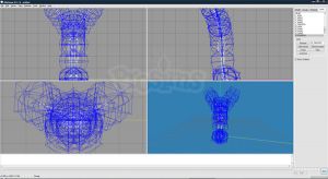
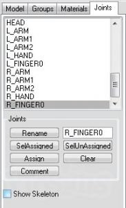
You will probably see something similar to the screenshot above. The blue outlines are the same information related to the movement of sims and in-game animations. It can be hidden by going to the "Joints" tab and unchecking "Show Skeleton".
Further, much rests on your experience with this program. I will try to talk about very basic actions.
To rotate the camera and thus view the mesh from all sides, hold down the left mouse button and move the cursor.
Right clicking on the window will give you a drop down list. If the checkbox is set to "Textured", you will see your mesh in volume. If it is on "Wireframe", you will see the wireframe mesh.

I suggest making the skirt a little longer.
In the menu on the right, select the “Model” tab and click on the “Select” button.
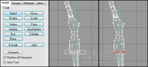
Just like you use the "Rectangular Marquee Tool" in Photoshop, select the points you want to move.

Right-click near the selected points, in the menu that opens, select "Frame Selection". This will bring the camera closer to the area you have selected and will result in a much cleaner result.
If the camera is too close, scroll the mouse wheel back and forth until the resulting angle suits you.
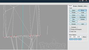
To the right of the "Select" button is "Move". Click it.
By holding the left mouse button and moving the cursor, move the points to the desired location. Remember that if you did something wrong (accidentally removed the selection or moved the points to the wrong place), you can always undo the last action by pressing Ctrl + Z.

Give the mesh a name
For an adult sim:
xskin-b (enter a 3-digit number) (put ma for an adult male or fa for an adult female) (put fit for a fit physique, fat for fat, or skn for thin) _ (enter a name for your mesh)-PELVIS-BODY.skn.
Example: xskin-B629MAFit_labtech-PELVIS-BODY.skn.
For a child:
xskin-b (enter a three-digit number) (put mc for a boy or fc for a girl) chd_ (enter a name for your mesh)-PELVIS-BODY.skn.
Example: xskin-b013mcchd_wizd-PELVIS-BODY.skn.
For the head:
xskin-c (enter a three-digit number) (put ma for adult male, fa for adult female, mc for boy, or fc for girl) _ (enter name for your mesh) -HEAD-HEAD.skn.
Example: xskin-c026fa_bwar-HEAD-HEAD.skn.
Create a link file
Open any text editor.
Insert the following text:
Save the resulting file with the .cmx extension.
The file will need to be given a name similar to the name of the skn-mesh, just remove the xskin- and -PELVIS-BODY (or -HEAD-HEAD) part from it.
Example:
Mesh xskin-b200fafit_bwar-PELVIS-BODY.skn and link file B200FAFit_BWar.cmx.
In order to compare, you can go to the GameData\Skins folder, open any cmx file with a text editor and look at its contents.
Give a name to the texture
This tutorial does not cover creating a texture, as it is dedicated to working with a mesh.
In order for the texture that you create for your mesh to be applied exactly to it, you need to give it an appropriate name.
For an adult sim:
b (enter a 3 digit number for your mesh) (put ma for a mature male or fa for a mature female) (put fit for a fit physique, fat for fat, or skn for thin) (put lgt for a light skin tone, med for a medium skin tone, or drk for a dark skin tone) _ (enter a name for your texture, it can be anything) .bmp.
Example: B022FAFitlgt_EAS.bmp.
For a child:
b (enter a three-digit number for your mesh) (put mc for a boy or fc for a girl) chd (put lgt for a light skintone, med for a medium skintone, or drk for a dark one) _ (enter a name for your texture, it can be anything) .bmp.
Example: B203FCChdLgt_CreepyMindy.bmp.
For the head:
c(enter a three-digit number for your mesh) (put ma for an adult male, fa for an adult female, mc for a boy, or fc for a girl) (put lgt for a light skintone, med for a medium skintone, or drk for a dark one)_(enter a name for your texture ).bmp.
Example: C481FAlgt_May.bmp.
A few last notes
When editing a mesh in Milkshape, never move, rotate, change or resize the entire mesh;
- One and the same mesh can correspond to any number of bmp-textures, the name of which ends differently;
- If the number you entered matches the number already in the game, a crash will occur. Because of this, your texture for the new mesh may be pulled over the standard mesh, or vice versa - one of the standard textures will jump to the mesh you created. If this happens, change the number in the skn, cmx and bmp files you created to another one.
Unfortunately, there is still no table on the Internet with a list of numbers already used for meshes in the game. However, there is such a table with the numbers of the meshes of the heads.
Despite this, Unity supports many 3D graphics packages. Unity also supports meshes that consist of both 3-sided and 4-sided polygons. Inhomogeneous rational bezier splines (Nurbs), inhomogeneous rationally smoothed meshes (Nurms) as well as high-poly surfaces must be converted to polygons.
3D formats
Importing meshes into Unity can be done using two main file types:
- Exported 3D file formats, such as .FBX or .OBJ
- Native 3D application files, such as .Max and .Blend files from 3D Studio Max and Blender.
Any of these types will allow you to add your own meshes to Unity, but there are considerations for which type you choose:
Exported 3D files
Advantages:
- Export only the data you need
- Checked data (before importing into Unity, re-import to the 3D package)
- Usually smaller files
- Supports a modular approach - for example different components for interactivity and collision types
- Supports other 3D packages whose formats are not directly supported by us
Flaws:
- Can slow down the process of prototyping and iteration
- It is easier to lose track between the original (working file) and the game version of the data (for example, an exported FBX file)
Native 3D application files
Unity can also import, by converting, files: Max, Maya, Blender, Cinema4D, Modo, light wave and Cheetah3D, for example, .MAX, .MB, .MA and etc.
Advantages:
- Fast iteration process (to re-import into Unity, save the original file)
- Initially simple
Flaws:
- The machines involved in the work on the Unity project must have licensed copies of this software installed
- Files containing unnecessary data can become unreasonably large
- Large files can slow down the autosave process
- Less checking, so it's harder to fix bugs
Here is a list of supported 3D graphics packages, others most often export the above mentioned file type.
Textures
When importing a mesh, Unity will try to use its search method to automatically find the textures used by it. The importer will first look for the Textures subfolder, either inside the mesh folder or in the folders one level up. If this does not help, then a global search will be performed throughout the entire project structure for all available textures. Of course, this search method is much slower than usual and its main disadvantage is that two or more textures with the same name may appear in the search results. In this case, there is no guarantee that the desired texture will be found.
Doc-menu">Textures in or above the level with components (assets)
Create and assign material
For each imported material, Unity will apply the following rules:-
If the material generation is canceled (in other words, if the Import Materials checkbox is not checked), then the default material will be assigned. If the generation was enabled, then the following will happen:
- Unity will use the name for its material based on the value of the Material Naming parameter
- Unity will try to find an existing material with that name. The search area for material search is set using the Material Search parameter
- If Unity manages to find an existing material, then it will be used in the imported scene, if not, then a new material will be created
Colliders
Unity uses two main types of colliders: Mesh Colliders and Primitive Colliders. Mesh colliders are those components that use the data of an imported mesh for themselves and can be used to create collisions with the environment. When you enable the Generate Colliders option in the Import Settings, the collider mesh will automatically be added to the scene along with the imported mesh. It will be considered complete as long as it works within the context of being used by a physical system.
When moving your object around the scene (like a car), you cannot use mesh colliders. Instead, you need to use primitive colliders. In this case, you need to disable the Generate Colliders option.
Animations
Animations are automatically imported from the scene. For more detailed information about animation import settings, visit the documentation chapter titled Preparing components and importing them in the animation system (Mecanim).
Normal mapping and characters
If you have a character model with a normal map applied to it, taken from a high poly model, then you will need to import into the scene a version of the model for playing with a Smoothing angle of 180 degrees. This way you can prevent strange-looking seams at the joints of the model. If the seams still remain even after applying these settings, then activate the option Split tangents across UV seams.
If you're converting a black and white image to a normal map, you don't have to worry about that.
Blendshapes
Unity supports Blendshapes (also called morph targets or vertex animations). Unity can import blend shapes from formats such as .FBX(blend shapes and animation controls) and .dae(mix shapes only). Unity blend shapes also support vertex animation on vertices, normals, and tangents. A mesh can be affected by both its Skin and blend shapes at the same time. All meshes that have been imported with blend shapes will use the SkinnedMeshRenderer component (whether it has been previously skinned or not). The blend shape animations are imported as part of the regular animation - it simply animates the weights of the blend shapes on the SkinnedMeshRenderer component.
There are two ways to import blend shapes with normals:
- If you set the Normals import mode to Calculate , then the same normal calculation sequence will be used for the meshes as for the blend shapes.
- Export information about smoothing groups to a source file. This way Unity will calculate the normals from the smoothing groups for both the mesh and blend shapes.
If you need tangents on your blend shapes, then set the Tangents import mode to Calculate .
- Merge together as many meshes as possible into a single whole. And make sure they use the same materials and textures. This should give a nice performance boost.
- If in the process of working in Unity you will often have to deal with setting up your objects (by applying physics, scripts and other useful things to them), then in order to save yourself from unnecessary headaches in the future, you should take care of the correct naming of your objects in advance 3D application in which they were originally created. Because how to work with a large number of objects that have names like pCube17 or Box42 to put it mildly, not very convenient.
- When working in your 3D application, try to position your models in the center of the world coordinate system. In the future, this will simplify their placement in Unity.
- If the vertices of the mesh initially do not have their own colors, then Unity will automatically assign white color to all vertices on the first render.
The Unity editor displays many more vertices and triangles (compared to what is displayed in my 3D application).
And there is. What you really need to pay attention to is how many vertices/triangles were actually sent to the GPU for rendering. Unlike in cases where the material requires that this data be sent to the GPU twice, things like hard-normals and non-contiguous UVs intentionally display a much larger number of vertices/triangles than there are on really. In the context of UV and 3D space, the triangles must be adjacent to form a border, so reducing the number of triangles at the UV seams that should have formed the border creates the effect of an imaginary increase in their number.
Attention, the lesson is not designed for beginners with zero knowledge in this matter! If you do not have basic skills in working in 3D programs, Workshop and Photoshop, then this tutorial will simply be useless for you. Learn at least texturing at the proper level, and learn how to minimally edit game meshes, and only then move on to more complex ones. To work, we need a set of individual body parts in obj format (Download), and, of course, any 3d program (I work in three for my own convenience - Milkshape, Khed and 3d Max, but one is enough for you). The tutorial is written using Milkshape. Since I am going to make women's clothing, namely a dress, we will use a female body mesh called afbody.obj (for reference: AF is the abbreviation for the adult female body mesh (Adult Female), AM is the adult male mesh (Adult Male), EF- EM - women's and men's meshes for the elderly, TF-TM - women's and men's meshes for teenagers, CU - mesh for children (Child Unisex), PU - mesh for toddlers (Puppy Unisex)).
So, the checkbox with Auto Smooth in the Groups section should be unchecked. Import the afbody.obj file into Milka (File – Import – Wavefront Object):
For convenience, we freeze the vertices so as not to accidentally deform the mesh. To do this, click on the Select panel, completely select the body and press Ctrl + H (or go to Edit - Hide Selection). Our model should turn gray:

It's time to create the skirt mesh itself. We hold down the mouse wheel and slightly move the mannequin to the side, then click on the Sphere panel and put down the values a little more than those that were originally there:

Of course, you can experiment with others as well. the higher the values, the smoother our sphere, but also more faces and polygons. Just find the best option for you. I didn't write too much in order not to complicate the lesson.

Only, of course, it doesn’t look like a skirt yet, so we cut off part of the sphere. To do this, select it using Select:

Press the Delete button on the keyboard:

The base of the skirt is ready. Again, fully select our hemisphere and drag it onto the model using Move. Arrange it the way we like it and get ready to dance the baboon dance, because we have almost created the mesh of our dress!

By the way, I show you all four projections for a reason. Pay attention that the center of our skirt is exactly in the middle of the body mesh, move it in all the windows.
Of course, I don't have a Victorian puffy skirt in my plans, so I want to make it a little smaller. To do this, click Scale and drive in the following values:

The larger the value, the larger the increase in the selected area. Be sure to press U in the list of coordinates (see screenshot above), otherwise the skirt will only decrease in the sides. After you have entered the numbers, click on the white Scale button:

If everything suits you, then you can skip the next part of the tutorial, but personally, I think that this skirt is unfinished.
Now it will be more convenient for me to work in a full window. Select the top left, press the right mouse button and select Maximize from the menu that opens. By the way, I want to ask you in advance to constantly enable these modes and window views from the same menu:

By default we have Wireframe set (we see just vertex points), switching to Smooth Shaded allows us to see the texture, like on a mannequin in the fourth window with 3D view. To see dots on this texture, click Wireframe Overlay. In the screenshot below we see the projections available to us, you can view the mesh from all sides by simply switching views.

I want to lengthen the skirt a little and give it a slightly elongated shape. Select each row of vertices and slightly lower it. You can also experiment with the size and splendor of the skirt, using Scale and driving in different values (if you want to reduce it a little, then write 0.9, 0.9, 0.9. If you increase it - 1.1, 1.1, 1.1).
I got this, uh ... pretty skirt:

You can see that I removed the closed top (although this is not necessary) and adjusted it with the Move and Scale tools to fit the waist. All rows of dots must be equidistant from each other! This is mandatory, otherwise the bones may not bind. Now it would be worth rounding the bottom so that it does not look like a solid line. Select the bottom row of points and slightly shift down:

Now select the points in the middle and move them too:

Then select the adjacent two points (each separately with the Shift key pressed), and move them.

We should get such charm:

Switch to left or right view mode. To be honest, I don't like that the skirt is so fluffy:

Therefore, we click on the coordinates we don’t need (look at the screen above - those that are gray), leave only Z active. Enter the values like mine, select the skirt and click on Scale as many times as our skirt becomes normal volume.

Of course, our top also decreased. If you switch to the front view mode, you can see this disgrace at the waist:

To make the edge more or less even, select it and enter the Scale values 1.1, 1.1, 1.1. We do not include any coordinates, press Scale as many times as we get smooth edges. We look through our mesh in all windows so that nothing extra comes out! Result:

The mesh is ready. We go into the groups and see that there are several of them:

Groups called GEOM are our mannequin. GEOM-00 - top, GEOM-01 - lower body. If you want to make a mesh for the upper part (jacket, tunic), then remove the bottom, if for the bottom (just a skirt, for example) - the top. Since we have a dress, we leave it as it is, just combine these parts of the mannequin (select both groups through Select, then Regroup). Now we need to create a texture scan (then you won’t be able to do this!), so we don’t merge anything into one group, but simply save our file in .obj format (File - Export - Wavefront Object). We do not close Milka, we just turn it off. Open UVMapper (download) and load our mesh (File – Load Model), we see this beauty:

Our skirt is not where we need it, so click Edit – Select – By Group. Select a group with a sphere:

The skirt should "turn red":

We move it to a place convenient for us, trying not to overlap the body scan (I placed a mannequin at hand) and scale it:

That's it, save our texture map (File – Save Texture Map) and the mesh itself (File – Save Model).
Open the mesh model saved after UVMapper in Milk. If you don't want the underside of the dress to be black, select the group with the skirt, duplicate (Edit - Duplicate Selection), then apply Face - Reverse Vertex Order to the duplicated skirt (if the underside is still black, then reduce the duplicated group a little using Scale) .

We now unite all our groups (Select - Regroup), rename the one and only to group_base (in the white field to the right of Rename, write a new name and press this very button)

Save the finished mesh in .wso format (File - Export - TSRW Object).
Now we need to bind the bones and create Fat, Thin and Fit physiques, for this we need MeshToolKit (download). But first, we open the Workshop and find a dress that looks like a mesh to ours. I chose pink

Export its mesh called Reference:

Now open MeshToolKit. I have marked three tabs that we will need:

We check the file:

We check the bones:

We do autobinding. Attention! Be careful, there is a small, but still a chance of incorrect binding!

We create physiques. It may take some time. Be sure to select our previous saved mesh with attached bones:

Ready! You can check the file in Milk:

As you can see, there are body groups, the bones are also tied.
Import the file into Work, into all mesh groups (High level of detail, etc.). On the first message that appears to us, click "No":

Then you can freely click "Yes".
Hooray! We created our OWN mesh:

Let's start working on the texture. Open our scan in Photoshop, and go to Image - Image Size, set 1024 * 1024:

Then again go to Image - Mode - RGB. Everything, you can start creating textures. I will not describe the process, because this lesson is designed for those who have long been accustomed to retexturing. As a rule, I'm more comfortable working without alpha channels, so don't be surprised if the background is transparent.
My texture is like this:


All the necessary operations have been done, but the final touch remains, MANDATORY for all creators who strive for quality and do not spit on those who download their content. Reduce the weight of the dress by removing the textures we don't need. In the work, click at the top of the panel Edit - Project Contents. In the new window, the DDS I highlighted are our textures. There should be 3-6 of them. Textures that were loaded earlier and turned out to be unnecessary are also saved there, check the files for their presence. Other extensions cannot be touched, only DDS!

If you need to use, for example, one Multiplier several times, then use the Browse button so that you do not constantly load the same texture and do not take up space with it:

Removing the excess, enter the original name and save. Checking in game:

Our work has been successfully completed. Good luck with your meshing!
Thank you for helping with Sintiklia information and for photographing the dress in the Misti game.
A similar technique is used to display MRI images, metaballs and for terrain voxelization.
In this part, I will talk about the Marching Cubes technique for creating a destructible relief, and in a more general application - for creating a smooth boundary mesh of a solid object. In this article, we will start by looking at 2D techniques, then 3D, and in the third part we will look at Dual Contouring. Dual Contouring is a more advanced technique that produces the same effect.
Our goal
First, let's define what we want to achieve. Suppose we have a function that can be discretized over the entire space, and we want to plot its boundary on the graph. In other words, determine where the function transitions from positive to negative and vice versa. In the breakable terrain example, we will interpret positive areas as solid and negative areas as empty. A function is a great way to describe an arbitrary shape. but it doesn't help us draw it.
To draw, we need to know it border, for example, the points between positive and negative values where the function crosses zero. The Marching Cubes algorithm takes such a function and creates a polygonal approximation of its boundary that can be used for rendering. In 2d this border will be a continuous line. When going to 3d, it becomes a mesh.
Implementation of 2D Marching Cubes
Note: python code, which contains commented code with everything you need. For simplicity, let's start with 2d and move on to 3d later. I will call the 2d and 3d algorithms "Marching Cubes" because they are essentially the same algorithm.
Step 1
First, we will divide the space into a uniform grid of squares (cells). Then, for each cell, we can use a function evaluation to determine whether each vertex of the cell is inside or outside the solid area. Below is a function that describes a circle, and black dots mark all vertices whose coordinates are positive.
Step 2
We then process each cell separately, filling it with the appropriate border.
A simple lookup table provides 16 possible combinations of corners, either outside or inside. In each case, it determines which border should be drawn.
All combinations of 2D marching cubesStep 3
After repeating the process for all cells, the borders are connected, creating a finished mesh, even though each cell was considered independently.
Excellent! I think it generally resembles the original circle described by the formula. But as you can see, it is all broken, and the segments are located at angles of 45 degrees. This happened because we decided to select the border vertices (red squares) equidistant from the cell points. adaptability
The best way to get rid of 45 degree corners would be adaptive marching cubes algorithm. Instead of simply defining all the border vertices from the center points of the cells, they can be positioned to best fit the solid area. To do this, we not only need to know whether a point is inside or outside; we also need to know how deep is it.This means that we need some kind of function that gives us a measure of how deep a point is inside/outside. It doesn't have to be exact because we only use it for approximations. In the case of our perfect circle, which has a radius of 2.5 units, we will apply the following function.
In which positive values are inside and negative values are outside. Then we can use the numerical values on either side of the face to determine how far along the face the point should be placed.
Putting it all together, it will look like this:
Even though we have the same vertices and lines as before, a slight change in position makes the resulting shape much more like a circle. Part 2. 3D Marching Cubes
So, in 2D, we grid space, and then for each vertex of the cell, we calculate whether that point is inside or outside the solid area. In a 2d grid, each square has 4 corners, and for each of them there are two options, that is, each cell has possible combinations of corner states. Then we fill the cell with our segment for each of the 16 cases, and all the segments of all cells naturally join together. We use adaptability to best fit these segments to the target surface.
Good news is that in the three-dimensional case, everything works almost the same way. We divide the space into a grid of cubes, consider them separately, draw some edges for each cube, and they connect, creating the desired border mesh.
Bad news is that the cube has 8 corners, that is, there are considered possible cases. And some of these cases are much more complex than in 2D.
Very good news is that we do not need to understand it at all. You can just copy the cases I've collected and jump straight to the results section ("Putting it all together") without having to think about all the complexities. And then start reading about dual contouring if you need a more powerful technique.
All difficulties
Note: this tutorial focuses more on concepts and ideas than implementation methods and code. If you're more interested in the implementation, check out the 3D python implementation, which contains the commented code with everything you need. Are you still reading? Great, I like it.
The secret is that we really not required collect all 256 different cases. Many of them are mirror images or rotations of each other.

Here are three different cases of cells. Red corners are solid, all others are empty. In the first case, the bottom corners are solid and the top corners are empty, so you need to split the cell vertically to render the dividing border correctly. For convenience, I've colored the outside of the border yellow and the inside blue. The remaining two cases can be found by simply rotating the first case.
We can use another trick:

These two cases are opposite to each other - the solid corners of one are empty of the other, and vice versa. We can easily generate one case from another - they have the same border, just reversed.
With all this in mind, in fact, we need to consider only 18 cases, from which we can generate all the rest.

The only sane person
If you read most of the Marching Cubes tutorials, they say that only 15 cases are needed. How so? Well, that's actually true - the bottom three cases from my diagram aren't necessarily needed. Here again these three cases are compared with other opposite cases that give a similar surface.
Both the second and third columns correctly separate solid corners from empty ones. But only when we consider one cube separately. If you look at the edges of each face of the cell, you can see that they are different for the second and third columns. The inverted ones will not properly connect to neighboring cells, leaving holes in the surface. After adding the extra three cases, all cells are correctly connected. Putting it all together
As in the 2D case, we can simply process all the cells independently. Here is a spherical mesh created from Marching Cubes.
As you can see, the shape of the sphere as a whole is done correctly, but in some parts there is a chaos of narrow generated triangles. You can solve this problem with the Dual Contouring algorithm, which is more advanced than Marching Cubes. Part 3 Dual Contouring
Marching Cubes are easy to implement, so they are often used. But the algorithm has many problems: 
What do we do?
Dual Contouring appears on the scene
Note: this tutorial focuses more on concepts and ideas than implementation methods and code. If you're more interested in the implementation, then check out the python implementation, which contains the commented code with everything you need ( and ). Dual Contouring solves these problems and is much more extensible in doing so. Its disadvantage is that we need even more information about , that is, about the function that determines what is solid and empty. We need to know not only the value, but also the gradient. This additional information will improve adaptability compared to marching cubes.
Dual Contouring puts one vertex in each cell and then "connects the dots" to create a complete mesh. The points are connected along each edge that has a sign change, just like in marching cubes.
Note: the word "dual" ("dual") in the name appeared because the cells in the grid become the vertices of the mesh, which connects us with dual graph .Unlike Marching Cubes, we cannot calculate cells individually. In order to "connect the dots" and find a complete mesh, we must look at neighboring cells. But it's actually a much simpler algorithm than Marching Cubes because there aren't many separate cases. We simply find each edge with a sign change and connect the vertices of the cells adjacent to this edge.
Getting the Gradient
In our simple 2d circle example, radius 2.5 is given as follows:
(in other words, 2.5 minus the distance from the center point) Using differential calculus, we can calculate the gradient:
The gradient is a pair of numbers for each point indicating how much the function changes as it moves along the x or y axis. But to get the gradient function, we do not need complex calculations. We can simply measure the change when and deviate by a small amount.
This will work for any smooth , as long as the chosen one is small enough. In practice, it turns out that even functions with sharp points turn out to be smooth enough, because in order for this to work, it is not necessary to calculate the gradient near the sharp sections. Link to code. adaptability
So far, we've got the same stepped look that the Marching Cubes had. We need to add adaptability. In the Marching Cubes algorithm, we chose where the vertex would be along the edge. Now we can freely choose any point of the interior of the cell. We want to choose the point that most closely matches the information we received, i.e. calculated value
And the gradient. Notice that we sampled the gradient along the edges, not the corners.
By choosing the point shown, we ensure that the rendered faces of that cell are as normal as possible:
In practice, not all normals in a cell will fit. We need to choose the most suitable point. In the last section, I will tell you how to choose this point. Going to 3d
The cases in 2d and 3d are not really very different. The cell is now a cube instead of a square. We're drawing faces, not edges. But that's where the differences end. The procedure for selecting one point in a cell is the same. And we still find the edges with a sign change, and then connect the points of neighboring cells, but now four cells, which gives us a four-sided polygon: 
A face associated with a single edge. She has dots in every adjacent cell.results
Dual contouring creates much more natural shapes than marching cubes, as can be seen in the sphere created with it:
In 3d, this procedure is robust enough to select points that are along the edge of a sharp section and select corners as they occur. Problems
Colinear Normals
Most tutorials stop there, but the algorithm has a dirty little secret - the QEF solution as described in the original Dual Contouring article doesn't actually work very well. By solving QEF, we can find the point that best fits the normals of the function. But really there is no guarantee that the resulting point is inside the cell.
In fact, quite often it is outside when we work with large flat surfaces. In this case, all sampled normals will be the same or very close, as in this figure.
I have seen many tips to solve this problem. Some people have given up by discarding the gradient information and using the center of the cell or the average of the border positions instead. It's called Surface Nets, and there's at least some simplicity to such a solution. Technique 1: QEF Solution with Constraints
Remember that we found the cell point by finding the point that minimizes the value of a given function called QEF. By making small changes, we can find the minimizing point inside cells. Technique 2: QEF bias
We can add any quadratic function to QEF and get another quadratic function that is still solvable. Therefore, I added a quadratic function that has a minimum point in the center of the cell. Due to this, the solution of the entire QEF contracts to the center.
In fact, this has more of an effect when the normals are collinear and is more likely to give poor results, but has little effect on positions in the good case.
Using both techniques is rather redundant, but in my opinion gives the best visual results.
Both techniques are shown in more detail in the code.
Self-intersections
Another issue with dual contouring is that it can sometimes generate a self-intersecting 3d surface. In most cases, this is ignored, so I did not solve this problem. There is an article that talks about her solution: "Intersection-free Contouring on An Octree Grid", Ju and Udeshi, 2006
Uniformity
Although the resulting dual contouring mesh is always airtight, the surface is not always well defined. Since there is only one point per cell, when two surfaces pass through the cell, it will be common to them. This is called a "uniform" mesh and can cause problems for some texturing algorithms. The problem often occurs when solid objects are thinner than the cell size, or when multiple objects are almost touching each other.
Handling such cases is a significant extension of the functionality of the basic Dual Contouring. If you need this feature, I recommend looking into this implementation of Dual Contouring, or Algorithm extension
Due to the relative ease of creating meshes, Dual Contouring is much easier to extend to work with cell layouts other than the standard meshes discussed above. In general, the algorithm can be run on octrees to get different cell sizes exactly where the details are needed. In general, the idea is similar - we select one point per cell using sampled normals, then for each edge with a sign change we find neighboring 4 cells and combine their vertices into a face. In an octree, you can use recursion to find these edges and neighboring cells. Matt Keeter has about it. Another interesting extension is that for Dual Contouring all we need is a definition of what is inside/outside and the corresponding normals. Although I said that we have a function for this, we can extract the same information from another mesh. This allows us to perform a "remesh", i.e. generate a clean set of vertices and faces that clean up the original mesh. An example is the remesh modifier from Blender.
Additional reading
- Dual Contouring is one of many similar techniques. See the SwiftCoder list for other approaches with their pros and cons.
Tags: Add tags