Elementary Matrix Transformations
Elementary matrix transformations are widely used in various mathematical problems. For example, they form the basis of the well-known Gauss method (method of eliminating unknowns) for solving a system of linear equations.
The elementary transformations are:
1) permutation of two rows (columns);
2) multiplication of all elements of the row (column) of the matrix by some number that is not equal to zero;
3) addition of two rows (columns) of a matrix multiplied by the same non-zero number.
The two matrices are called equivalent, if one of them can be obtained from the other after a finite number of elementary transformations. In general, equivalent matrices are not equal, but have the same rank.
Calculation of determinants using elementary transformations
Using elementary transformations, it is easy to calculate the matrix determinant. For example, it is required to calculate the matrix determinant:
where ≠ 0.
Then you can take out the multiplier:

now, subtracting from the elements j-th column, the corresponding elements of the first column, multiplied by, we get the determinant:

which is: where


Then we repeat the same steps for and if all elements ![]() then we finally get:
then we finally get:

If for some intermediate determinant it turns out that its upper left element is , then it is necessary to rearrange the rows or columns so that the new upper left element is not equal to zero. If ∆ ≠ 0, then it can always be done. In this case, it should be taken into account that the sign of the determinant changes depending on which element is the main one (that is, when the matrix is transformed in such a way that). Then the sign of the corresponding determinant is equal.
EXAMPLE Using elementary transformations, bring the matrix
Elementary matrix transformations are such transformations of the matrix , as a result of which the equivalence of matrices is preserved. Thus elementary transformations do not change the solution set of the system of linear algebraic equations that this matrix represents.
Elementary transformations are used in the Gauss method to bring a matrix to a triangular or stepped form.
Definition
Elementary string transformations called:
In some linear algebra courses, a permutation of matrix rows is not distinguished as a separate elementary transformation due to the fact that a permutation of any two matrix rows can be obtained using the multiplication of any matrix row by a constant k (\displaystyle k), and adding to any row of the matrix another row, multiplied by a constant k (\displaystyle k), k ≠ 0 (\displaystyle k\neq 0).
The elementary column transformations.
Elementary transformations reversible.
The notation indicates that the matrix A (\displaystyle A) can be obtained from B (\displaystyle B) by elementary transformations (or vice versa).
Properties
Rank invariance under elementary transformations
| Theorem (on rank invariance under elementary transformations). If A ∼ B (\displaystyle A\sim B), then r a n g A = r a n g B (\displaystyle \mathrm (rang) A=\mathrm (rang) B). |
Equivalence of SLAE under elementary transformations
Let's call elementary transformations over a system of linear algebraic equations :- permutation of equations;
- multiplying an equation by a non-zero constant;
- addition of one equation to another, multiplied by some constant.
Finding inverse matrices
| Theorem (on finding the inverse matrix). Let the matrix determinant A n × n (\displaystyle A_(n\times n)) is not equal to zero, let the matrix B (\displaystyle B) is defined by the expression B = [ A | E ] n × 2 n (\displaystyle B=_(n\times 2n)). Then, under an elementary transformation of the rows of the matrix A (\displaystyle A) to identity matrix E (\displaystyle E) as part of B (\displaystyle B) transformation takes place at the same time. E (\displaystyle E) To A − 1 (\displaystyle A^(-1)). |
Elementary matrix transformations are widely used in various mathematical problems. For example, they form the basis of the well-known Gauss method (method of eliminating unknowns) for solving a system of linear equations.
The elementary transformations are:
1) permutation of two rows (columns);
2) multiplication of all elements of the row (column) of the matrix by some number that is not equal to zero;
3) addition of two rows (columns) of a matrix multiplied by the same non-zero number.
The two matrices are called equivalent, if one of them can be obtained from the other after a finite number of elementary transformations. In general, equivalent matrices are not equal, but have the same rank.
Calculation of determinants using elementary transformations
Using elementary transformations, it is easy to calculate the matrix determinant. For example, it is required to calculate the matrix determinant:
Then you can take out the multiplier:
now, subtracting from the elements j th column, the corresponding elements of the first column, multiplied by , we get the determinant:
which is: where
Then we repeat the same steps for and, if all elements then we finally get:
If for some intermediate determinant it turns out that its upper left element is , then it is necessary to rearrange the rows or columns in so that the new upper left element is not equal to zero. If ∆ ≠ 0, then it can always be done. In this case, it should be taken into account that the sign of the determinant changes depending on which element is the main one (that is, when the matrix is transformed so that ). Then the sign of the corresponding determinant is .
EXAMPLE Using elementary transformations, bring the matrix
to a triangular shape.
Solution: First, multiply the first row of the matrix by 4 and the second row by (-1) and add the first row to the second:
Now multiply the first row by 6 and the third by (-1) and add the first row to the third:
Finally, multiply the 2nd row by 2 and the 3rd row by (-9) and add the second row to the third:
The result is an upper triangular matrix
Example. Solve a system of linear equations using the matrix apparatus:
Solution. We write this system of linear equations in matrix form:
The solution of this system of linear equations in matrix form has the form:
where is the matrix inverse to the matrix A.
Coefficient matrix determinant A equals:
hence the matrix A has an inverse matrix.
2. Maltsev A.I. Fundamentals of linear algebra. – M.: Nauka, 1975. – 400 p.
3. Bronstein I.N., Semendyaev K.A. Handbook of mathematics for engineers and students of higher educational institutions. – M.: Nauka, 1986. – 544 p.
Let us introduce the concept of an elementary matrix.
DEFINITION. The square matrix obtained from the identity matrix as a result of a non-singular elementary transformation over rows (columns) is called the elementary matrix corresponding to this transformation.
For example, the second-order elementary matrices are the matrices
where A is any nonzero scalar.
The elementary matrix is obtained from the identity matrix E as a result of one of the following non-singular transformations:
1) multiplication of a row (column) of the matrix E by a non-zero scalar;
2) addition (or subtraction) to any row (column) of the matrix E of another row (column), multiplied by a scalar.
Denote by the matrix obtained from the matrix E as a result of multiplying a row by a non-zero scalar A:

Denote by the matrix obtained from the matrix E as a result of adding (subtracting) to the row of the row multiplied by A;

Through we will denote the matrix obtained from the identity matrix E as a result of applying an elementary transformation over rows; thus there is a matrix corresponding to the transformation
Consider some properties of elementary matrices.
PROPERTY 2.1. Any elementary matrix is invertible. A matrix inverse to an elementary one is elementary.
Proof. A direct verification shows that for any non-zero scalar A. and arbitrary ones, the equalities
Based on these equalities, we conclude that property 2.1 holds.
PROPERTY 2.2. The product of elementary matrices is an invertible matrix.
This property follows directly from Property 2.1 and Corollary 2.3.
PROPERTY 2.3. If a non-singular row elementary transformation transforms -matrix A into matrix B, then . The absurd statement is also true.
Proof. If there is a multiplication of a string by a non-zero scalar A, then

If , then

It is easy to verify that the converse is also true.
PROPERTY 2.4. If the matrix C is obtained from the matrix A using a chain of nonsingular row elementary transformations , then . The converse is also true.
Proof. By property 2.3, the transformation transforms the matrix A into a matrix, transforms the matrix into a matrix, etc. Finally, transforms the matrix into a matrix Therefore, .
It is easy to verify that the converse is also true. Matrix invertibility conditions. The following three lemmas are needed to prove Theorem 2.8.
LEMMA 2.4. A square matrix with a zero row (column) is not invertible.
Proof. Let A be a square matrix with row zero, B any matrix, . Let be the zero row of the matrix A; then
i.e., the i-th row of the matrix AB is zero. Therefore, the matrix A is irreversible.
LEMMA 2.5. If the rows of a square matrix are linearly dependent, then the matrix is not invertible.
Proof. Let A be a square matrix with linearly dependent rows. Then there is a chain of non-singular row elementary transformations that transform A into a step matrix; let such a chain. By property 2.4 of elementary matrices, we have
where C is a matrix with a zero row.
Therefore, by Lemma 2.4, the matrix C is not invertible. On the other hand, if the matrix A were invertible, then the product on the left in equality (1) would be an invertible matrix, like the product of invertible matrices (see Corollary 2.3), which is impossible. Therefore, the matrix A is irreversible.
The next three operations are called elementary transformations of matrix rows:
1) Multiplication of the i-th row of the matrix by the number λ ≠ 0:
which we will write in the form (i) → λ(i).
2) Permutation of two rows in the matrix, for example the i-th and k-th rows:
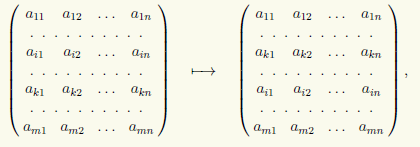
which we will write in the form (i) ↔ (k).
3) Adding to the i-th row of the matrix its k-th row with the coefficient λ:

which will be written in the form (i) → (i) + λ(k).
Similar operations on the columns of a matrix are called elementary column transformations.
Every elementary row or column transformation of a matrix has inverse elementary transformation, which transforms the transformed matrix into the original one. For example, the inverse transformation for permuting two strings is permuting the same strings.
Each elementary transformation of the rows (columns) of the matrix A can be interpreted as a left (right) multiplication of A by a matrix of a special form. This matrix is obtained if the same transformation is performed on identity matrix. Let us consider elementary string transformations in more detail.
Let the matrix B be obtained by multiplying the i-th row of an m × n matrix A by the number λ ≠ 0. Then B = Е i (λ)А, where the matrix Е i (λ) is obtained from the identity matrix E of order m by multiplying its i -th row by the number λ.
Let matrix B be obtained as a result of permutation of the i-th and k-th rows of an m×n matrix A. Then B = F ik A, where the matrix F ik is obtained from the identity matrix E of order m by interchanging its i-th and k-th rows.
Let the matrix B be obtained by adding to the i-th row of the m×n matrix A its k-th row with the coefficient λ. Then B = G ik (λ)А, where the matrix G ik is obtained from the identity matrix E of order m as a result of adding the kth row to the i-th row with the coefficient λ, i.e. at the intersection of the i-th row and the k-th column of the matrix E, the zero element is replaced by the number λ.
In the same way, elementary transformations of the columns of the matrix A are implemented, but at the same time it is multiplied by matrices of a special type not from the left, but from the right.
With the help of algorithms that are based on elementary transformations of rows and columns, matrices can be transformed to a different form. One of the most important such algorithms forms the basis of the proof of the following theorem.
Theorem 10.1. Using elementary row transformations, any matrix can be reduced to stepped view.
◄ The proof of the theorem consists in constructing a specific algorithm for reducing a matrix to a stepped form. This algorithm consists in multiple repetitions in a certain order of three operations associated with some current element of the matrix, which is selected based on the location in the matrix. At the first step of the algorithm, we choose the upper left element as the current element of the matrix, i.e. [A] 11 .
one*. If the current element is zero, go to operation 2*. If it is not equal to zero, then the row in which the current element (the current row) is located is added with the appropriate coefficients to the rows located below, so that all matrix elements in the column under the current element turn to zero. For example, if the current element is [A] ij , then as the coefficient for the kth row, k = i + 1, ... , we should take the number - [A] kj /[A] ij . We select a new current element, shifting in the matrix one column to the right and one line down, and proceed to the next step, repeating operation 1*. If such a shift is not possible, i.e. the last column or row is reached, we stop converting.
2*. If the current element in some row of the matrix is equal to zero, then we look at the matrix elements located in the column under the current element. If there are no non-zero ones among them, we pass to operation 3*. Let there be a non-zero element in the k-th line under the current element. Swap current and k-th lines and return to operation 1*.
3*. If the current element and all elements below it (in the same column) are equal to zero, change the current element by shifting one column to the right in the matrix. If such a shift is possible, i.e. the current element is not in the rightmost column of the matrix, then repeat the operation 1* . If we have already reached the right edge of the matrix and changing the current element is not possible, then the matrix has a stepped form, and we can stop the transformations.
Since the matrix has finite dimensions, and in one step of the algorithm the position of the current element is shifted to the right by at least one column, the transformation process will end, and in no more than n steps (n is the number of columns in the matrix). This means that there will come a time when the matrix will have a stepped form.
Example 10.10. Let's transform the matrix  to a stepped form with the help of elementary string transformations.
Using the algorithm from the proof of Theorem 10.1 and writing the matrices after the completion of its operations, we obtain