Distributed computing gpu. GPU optimization - common truths. Using GPU resources to the full - GPU Occupancy

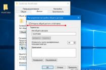
GPU Computing with C++ AMP

So far, in the discussion of parallel programming techniques, we have considered only processor cores. We have gained some skills in parallelizing programs across multiple processors, synchronizing access to shared resources, and using high-speed synchronization primitives without the use of locks.

However, there is another way to parallelize programs - graphics processing units (GPUs), which have more cores than even high-end processors. GPU cores are great for implementing parallel data processing algorithms, and their large number more than compensates for the inconvenience of running programs on them. In this article, we will get acquainted with one of the ways to execute programs on the GPU, using a set of C ++ language extensions called C++AMP.

The C++ AMP extensions are based on the C++ language, which is why this article will show examples in C++. However, with moderate use of the mechanism of interactions in. NET, you will be able to use C++ AMP algorithms in your .NET programs. But we will talk about this at the end of the article.

Introduction to C++ AMP

In essence, a GPU is a processor like any other, but with a special set of instructions, a large number of cores, and its own memory access protocol. However, there are big differences between modern graphics processors and conventional processors, and understanding them is the key to creating programs that effectively use the computing power of the graphics processor.

Modern GPUs have a very small instruction set. This implies some limitations: the inability to call functions, a limited set of supported data types, the absence of library functions, and others. Some operations, such as conditional jumps, can cost significantly more than similar operations performed on conventional processors. Obviously, porting large amounts of code from the CPU to the GPU under these conditions requires a lot of effort.

The number of cores in the average GPU is significantly higher than in the average conventional processor. However, some tasks are too small or do not allow themselves to be broken down into a large enough number of pieces to benefit from the use of the GPU.

Synchronization support between GPU cores performing the same task is very scarce, and completely absent between GPU cores performing different tasks. This circumstance requires synchronization of the GPU with a conventional processor.

The question immediately arises, what tasks are suitable for solving on a GPU? Keep in mind that not every algorithm is suitable for running on a GPU. For example, GPUs don't have access to I/O devices, so you can't improve the performance of a program that retrieves RSS feeds from the Internet by using the GPU. However, many computational algorithms can be transferred to the GPU and their massive parallelization can be ensured. Below are a few examples of such algorithms (this list is by no means exhaustive):

image sharpening and sharpening, and other transformations;

fast Fourier transform;

transposition and matrix multiplication;

sorting numbers;

hash inversion "on the forehead".

A great source for more examples is the Microsoft Native Concurrency Blog, which provides code snippets and explanations for various algorithms implemented in C++ AMP.

C++ AMP is a framework included with Visual Studio 2012 that gives C++ developers an easy way to perform GPU computing and requires only a DirectX 11 driver. Microsoft has released C++ AMP as an open specification that any compiler vendor can implement.

The C++ AMP framework allows you to execute code on graphics accelerators, which are computing devices. Using the DirectX 11 driver, the C++ AMP framework dynamically detects all accelerators. C++ AMP also includes a software accelerator emulator and a conventional processor-based emulator, WARP, which serves as a fallback on systems without a GPU or with a GPU but lacks a DirectX 11 driver and uses multiple cores and SIMD instructions.

And now let's start exploring an algorithm that can be easily parallelized to run on a GPU. The implementation below takes two vectors of the same length and computes a pointwise result. It's hard to imagine anything more straightforward:

Void VectorAddExpPointwise(float* first, float* second, float* result, int length) ( for (int i = 0; i< length; ++i) { result[i] = first[i] + exp(second[i]); } }

To parallelize this algorithm on a conventional processor, it is required to split the range of iterations into several subranges and start one thread of execution for each of them. We've spent quite a bit of time in previous articles on exactly this way of parallelizing our first prime number search example - we've seen how to do it by manually creating threads, passing jobs to a thread pool, and using Parallel.For and PLINQ to automatically parallelize. Recall also that when parallelizing similar algorithms on a conventional processor, we took special care not to split the task into too small tasks.

For the GPU, these warnings are not needed. GPUs have many cores that execute threads very quickly, and the cost of a context switch is much lower than conventional CPUs. Following is the snippet trying to use the function parallel_for_each from the C++ AMP framework:

#include #include using namespace concurrency; void VectorAddExpPointwise(float* first, float* second, float* result, int length) ( array_view avFirst(length, first); array_view avSecond(length, seconds); array_view avResult(length, result); avResult.discard_data(); parallel_for_each(avResult.extent, [=](index<1>i) restrict(amp) ( avResult[i] = avFirst[i] + fast_math::exp(avSecond[i]); )); avResult.synchronize(); )

Now let's examine each part of the code separately. Note right away that the general form of the main loop has been retained, but the for loop originally used has been replaced by a call to the parallel_for_each function. In fact, the principle of converting a loop into a function or method call is not new to us - this technique has already been demonstrated using the Parallel.For() and Parallel.ForEach() methods from the TPL library.

Next, the input data (parameters first, second and result) are wrapped with instances array_view. The array_view class is used to wrap the data passed to the GPU (accelerator). Its template parameter defines the data type and its dimension. In order to execute instructions on the GPU that access data originally processed on a regular CPU, someone or something must take care of copying the data to the GPU, because most modern graphics cards are separate devices with their own memory. Array_view instances solve this problem - they ensure that data is copied on demand and only when they are really needed.

When the GPU completes the job, the data is copied back. By instantiating array_view with a const type argument, we ensure that first and second are copied into GPU memory, but not copied back. Likewise, calling discard_data(), we exclude copying result from the memory of a conventional processor to the memory of the accelerator, but this data will be copied in the opposite direction.

The parallel_for_each function takes an extent object that specifies the form of the data to be processed and the function to apply to each element in the extent object. In the example above, we used a lambda function, support for which was introduced in the ISO C++2011 (C++11) standard. The restrict (amp) keyword instructs the compiler to check that the function body can be executed on the GPU and disables most of the C++ syntax that cannot be compiled into GPU instructions.

lambda function parameter, index<1>object represents a one-dimensional index. It must match the extent object being used - if we were to declare the extent object to be two-dimensional (for example, defining the shape of the source data as a two-dimensional matrix), the index would also need to be two-dimensional. An example of such a situation is given below.

Finally, the method call synchronize() at the end of the VectorAddExpPointwise method, it ensures that the results of calculations from array_view avResult performed by the GPU are copied back to the result array.

This concludes our first introduction to the world of C++ AMP, and we are now ready for more detailed explorations, as well as more interesting examples that demonstrate the benefits of using parallel computing on the GPU. Vector addition is not the best algorithm and not the best candidate for demonstrating GPU usage due to the large data copy overhead. The next subsection will show two more interesting examples.

Matrix multiplication

The first "real" example we'll look at is matrix multiplication. For implementation, we will take a simple cubic algorithm for matrix multiplication, and not the Strassen algorithm, which has a runtime close to cubic ~O(n 2.807). Given two matrices, an m x w matrix A and a w x n matrix B, the following program will multiply them and return the result, an m x n matrix C:

Void MatrixMultiply(int* A, int m, int w, int* B, int n, int* C) ( for (int i = 0; i< m; ++i) { for (int j = 0; j < n; ++j) { int sum = 0; for (int k = 0; k < w; ++k) { sum += A * B; } C = sum; } } }

There are several ways to parallelize this implementation, and if you want to parallelize this code to run on a normal processor, the right choice would be to parallelize the outer loop. However, the GPU has a sufficiently large number of cores, and by parallelizing only the outer loop, we will not be able to create a sufficient number of tasks to load all the cores with work. So it makes sense to parallelize the two outer loops while leaving the inner loop untouched:

Void MatrixMultiply (int* A, int m, int w, int* B, int n, int* C) ( array_view avA(m, w, A); array_view avB(w, n, B); array_view avC(m, n, C); avC.discard_data(); parallel_for_each(avC.extent, [=](index<2>idx) restrict(amp) ( int sum = 0; for (int k = 0; k< w; ++k) { sum + = avA(idx*w, k) * avB(k*w, idx); } avC = sum; }); }

This implementation still closely resembles the sequential implementation of the matrix multiplication and vector addition example above, except for the index, which is now two-dimensional and available in the inner loop using the . How much faster is this version than the sequential alternative running on a conventional processor? Multiplying two 1024 x 1024 matrices (integers) the serial version on a regular CPU takes an average of 7350 milliseconds, while the GPU version - hold on tight - is 50 milliseconds, 147 times faster!

Simulation of particle motion

The examples of solving problems on the GPU presented above have a very simple implementation of the inner loop. It is clear that this will not always be the case. The Native Concurrency blog linked above demonstrates an example of modeling gravitational interactions between particles. The simulation includes an infinite number of steps; at each step, new values ​​of the elements of the acceleration vector for each particle are calculated and then their new coordinates are determined. Here, the vector of particles is subjected to parallelization - with a sufficiently large number of particles (from several thousand and more), you can create a sufficiently large number of tasks to load all the cores of the GPU.

The basis of the algorithm is the implementation of determining the result of interactions between two particles, as shown below, which can be easily transferred to the GPU:

// here float4 are vectors with four elements, // representing the particles involved in the operations void bodybody_interaction (float4& acceleration, const float4 p1, const float4 p2) restrict(amp) ( float4 dist = p2 - p1; // w is not here uses float absDist = dist.x*dist.x + dist.y*dist.y + dist.z*dist.z; float invDist = 1.0f / sqrt(absDist); float invDistCube = invDist*invDist*invDist; acceleration + = dist*PARTICLE_MASS*invDistCube; )

The initial data at each modeling step is an array with the coordinates and velocities of the particles, and as a result of the calculations, a new array is created with the coordinates and velocities of the particles:

Struct particle ( float4 position, velocity; // implementations of constructor, copy constructor, and // operator = with restrict(amp) omitted to save space ); void simulation_step(array & previous, array & next, int bodies) ( extent<1>ext(bodies); parallel_for_each (ext, [&](index<1>idx) restrict(amp) ( particle p = previous; float4 acceleration(0, 0, 0, 0); for (int body = 0; body< bodies; ++body) { bodybody_interaction (acceleration, p.position, previous.position); } p.velocity + = acceleration*DELTA_TIME; p.position + = p.velocity*DELTA_TIME; next = p; }); }

With the help of an appropriate graphical interface, simulation can be very interesting. The full example provided by the C++ AMP development team can be found on the Native Concurrency Blog. On my system with an Intel Core i7 processor and a Geforce GT 740M graphics card, 10,000 particle motion simulation runs at ~2.5 frames per second (steps per second) using the serial version running on a regular processor and 160 frames per second using the optimized the version running on the GPU is a huge performance boost.

Before wrapping up this section, there is one more important feature of the C++ AMP framework that can further improve the performance of code running on the GPU. GPUs support programmable data cache(often called shared memory). The values ​​stored in this cache are shared by all threads of execution in the same tile. Thanks to memory tiling, programs based on the C++ AMP framework can read data from the graphics card's memory into the shared memory of the tile and then access it from multiple threads of execution without re-retrieving the data from the graphics card's memory. Accessing shared tile memory is approximately 10 times faster than accessing graphics card memory. In other words, you have reasons to keep reading.

To provide a tiled version of the parallel loop, the parallel_for_each method is passed tiled_extent domain, which divides the multidimensional extent object into multidimensional tiles, and the tiled_index lambda parameter, which specifies the global and local ID of the thread within the tile. For example, a 16x16 matrix can be divided into 2x2 tiles (as shown in the figure below) and then passed to the parallel_for_each functions:

Extent<2>matrix(16,16); tiled_extent<2,2>tiledMatrix = matrix.tile<2,2>(); parallel_for_each (tiledMatrix, [=](tiled_index<2,2>idx) restrict(amp) ( // ... ));

Each of the four threads of execution that belong to the same tile can share the data stored in the block.

When performing operations with matrices, in the GPU core, instead of the standard index<2>, as in the examples above, you can use idx.global. Proper use of local tiling and local indexes can provide significant performance gains. To declare tiled memory shared by all threads of execution in a single tile, local variables can be declared with the tile_static specifier.

In practice, the method of declaring shared memory and initializing its individual blocks in different threads of execution is often used:

Parallel_for_each(tiledMatrix, [=](tiled_index<2,2>idx) restrict(amp) ( // 32 bytes shared by all threads in tile_static block int local; // assign value to element for this thread of execution local = 42; ));

Obviously, any benefit from using shared memory can only be obtained if access to this memory is synchronized; that is, threads should not access memory until it has been initialized by one of them. Synchronization of threads in a mosaic is done using objects tile_barrier(reminiscent of the Barrier class from the TPL library) - they can continue execution only after calling the tile_barrier.Wait () method, which will return control only when all threads call tile_barrier.Wait. For instance:

Parallel_for_each (tiledMatrix, (tiled_index<2,2>idx) restrict(amp) ( // 32 bytes shared by all threads in a tile_static block int local; // assign a value to an element for this thread of execution local = 42; // idx.barrier - instance of tile_barrier idx.barrier.wait(); // Now this thread can access the "local" array // using indexes of other threads of execution! ));

Now is the time to translate the acquired knowledge into a concrete example. Let's return to the implementation of matrix multiplication, performed without the use of tiled memory organization, and add the described optimization to it. Let's say that the size of the matrix is ​​a multiple of 256 - this will allow us to work with blocks of 16 x 16. The nature of matrices allows the possibility of block-by-block multiplication, and we can take advantage of this feature (in fact, dividing matrices into blocks is a typical optimization of the matrix multiplication algorithm, providing a more efficient cpu cache usage).

The essence of this approach is as follows. To find C i,j (element in row i and column j in the result matrix), we need to calculate the dot product between A i,* (i-th row of the first matrix) and B *,j (j-th column in the second matrix ). However, this is equivalent to calculating the partial dot products of the row and column and then summing the results. We can use this circumstance to transform the matrix multiplication algorithm into a tiled version:

Void MatrixMultiply(int* A, int m, int w, int* B, int n, int* C) ( array_view avA(m, w, A); array_view avB(w, n, B); array_view avC(m, n, C); avC.discard_data(); parallel_for_each(avC.extent.tile<16,16>(), [=](tiled_index<16,16>idx) restrict(amp) ( int sum = 0; int localRow = idx.local, localCol = idx.local; for (int k = 0; k

The essence of the described optimization is that each thread in the mosaic (256 threads are created for a 16 x 16 block) initializes its element in 16 x 16 local copies of fragments of the original matrices A and B. Each thread in the mosaic requires only one row and one column of these blocks, but all threads together will access each row and each column 16 times. This approach significantly reduces the number of accesses to the main memory.

To calculate the element (i,j) in the result matrix, the algorithm needs the complete i-th row of the first matrix and the j-th column of the second matrix. When the flows are tiled 16x16 represented in the diagram and k=0, the shaded areas in the first and second matrices will be read into shared memory. The thread of execution that computes element (i,j) in the result matrix will compute the partial dot product of the first k elements from the i-th row and the j-th column of the original matrices.

In this example, tiling provides a huge performance boost. The tiled version of matrix multiplication is much faster than the simple version, taking about 17 milliseconds (for the same original 1024 x 1024 matrices), which is 430 times faster than the normal CPU version!

Before we end our discussion of the C++ AMP framework, we'd like to mention the tools (in Visual Studio) available to developers. Visual Studio 2012 offers a debugger for the graphics processing unit (GPU) that allows you to set breakpoints, examine the call stack, read and change the values ​​of local variables (some accelerators support GPU debugging directly; for others, Visual Studio uses a software simulator), and a profiler that allows you to evaluate the benefits that an application receives from parallelization of operations using a GPU. For more information about the debugging features in Visual Studio, see the Walkthrough. Debugging a C++ AMP Application" on MSDN.

Alternatives to GPU Computing in .NET

So far, this article has only shown examples in C++, but there are several ways to harness the power of the GPU in managed applications. One way is to use interop tools that allow you to offload GPU core work to low-level C++ components. This solution is great for those who want to use the C++ AMP framework or have the ability to use out-of-the-box C++ AMP components in managed apps.

Another way is to use a library that works directly with the GPU from managed code. Several such libraries currently exist. For example, GPU.NET and CUDAfy.NET (both are commercial offerings). The following is an example from the GPU.NET GitHub repository demonstrating the implementation of the dot product of two vectors:

Public static void MultiplyAddGpu(double a, double b, double c) ( int ThreadId = BlockDimension.X * BlockIndex.X + ThreadIndex.X; int TotalThreads = BlockDimension.X * GridDimension.X; for (int ElementIdx = ThreadId; ElementIdx

I'm of the opinion that it's much easier and more efficient to learn a language extension (powered by C++ AMP) than trying to orchestrate library-level interactions or make significant changes to the IL language.

So, after we looked at the possibilities of parallel programming in .NET and using the GPU, no one doubts that the organization of parallel computing is an important way to improve performance. In many servers and workstations around the world, the invaluable computing power of conventional and GPU processors remains unused, because applications simply do not use them.

The Task Parallel Library gives us a unique opportunity to include all available CPU cores, although this will have to solve some of the most interesting problems of synchronization, excessive fragmentation of tasks, and unequal distribution of work between threads of execution.

The C++ AMP framework and other multi-purpose GPU parallel libraries can be successfully used to parallelize computations across hundreds of GPU cores. Finally, there is a previously unexplored opportunity to gain performance from the use of distributed computing cloud technologies, which have recently become one of the main directions in the development of information technology.

What software is needed to mine cryptocurrency? What to consider when choosing equipment for mining? How to mine bitcoins and ethereum using a video card on a computer?

It turns out that not only fans of spectacular computer games need powerful video cards. Thousands of users around the world use graphics cards to earn cryptocurrency! From several cards with powerful processors miners create farms- computing centers that extract digital money almost out of thin air!

Denis Kuderin is with you - an expert of the HeatherBober magazine on finance and their competent multiplication. I will tell you what it is mining on video card in 17-18 years, how to choose the right device for earning cryptocurrency, and why it is no longer profitable to mine bitcoins on video cards.

You will also learn where to buy the most productive and powerful video card for professional mining, and get expert tips to improve the efficiency of your mining farm.

1. Mining on a video card - easy money or unjustified expenses

A good video card is not just a digital signal adapter, but also a powerful processor capable of solving the most complex computing problems. And including - calculate the hash code for the block chain (blockchain). This makes graphics cards ideal for mining- Cryptocurrency mining.

Question: Why the graphics processor? After all, in any computer there is a central processing unit? Isn't it logical to do calculations with it?

Answer: The CPU processor can also calculate blockchains, but it does it hundreds of times slower than the video card processor (GPU). And not because one is better, the other is worse. They just work differently. And if you combine several video cards, the power of such a computing center will increase several times more.

For those who have no idea about how digital money is mined, a small educational program. Mining - the main, and sometimes the only way to produce cryptocurrency.

Since no one mints or prints this money, and they are not a material substance, but a digital code, someone must calculate this code. This is what miners do, or rather, their computers.

In addition to code calculations, mining performs several more important tasks:

• system decentralization support: lack of attachment to servers - the basis of the blockchain;
• transaction confirmation– without mining, operations will not be able to enter a new block;
• formation of new blocks of the system- and entering them into a single registry for all computers.

I want to immediately cool the ardor of novice miners: the mining process is becoming more and more difficult every year. For example, using a video card has long been unprofitable.

Bitcoins with the help of GPUs are now mined only by stubborn amateurs, since specialized processors have replaced video cards ASIC. These chips consume less electricity and are more efficient in terms of computing. All good, but worth the order 130-150 thousand rubles .

Powerful model Antminer S9

Fortunately for miners, bitcoin is not the only cryptocurrency on the planet, but one of hundreds. Other digital money - Ethereum, Zcash, Expanse, dogecoins etc. it is still profitable to mine with the help of video cards. The remuneration is stable, and the equipment pays off in about 6-12 months.

But there is another problem - the lack of powerful video cards. The excitement around the cryptocurrency has led to a rise in the price of these devices. It is not so easy to buy a new video card suitable for mining in Russia.

Novice miners have to order video adapters in online stores (including foreign ones) or purchase second-hand goods. By the way, I do not recommend doing the latter: Mining equipment becomes obsolete and wears out at a fantastic rate.

Avito even sells entire farms for cryptocurrency mining.

There are many reasons: some miners have already “played enough” in the extraction of digital money and decided to engage in more profitable operations with cryptocurrency (in particular, stock trading), others realized that they could not compete with powerful Chinese clusters operating on the basis of power plants. Still others switched from video cards to ASICs.

However, the niche still brings some profit, and if you start with the help of a video card right now, you will still have time to jump on the bandwagon of the train leaving for the future.

Another thing is that there are more and more players on this field. Moreover, the total number of digital coins does not increase from this. On the contrary, the reward becomes smaller.

So, six years ago, the reward for one blockchain of the Bitcoin network was equal to 50 coins, now it's only 12.5 BTK. The complexity of calculations thus increased by 10 thousand times. True, the cost of bitcoin itself has grown many times during this time.

2. How to mine cryptocurrency using a video card - step by step instructions

There are two mining options - solo and as part of a pool. It is difficult to engage in single production - you need to have a huge amount of hashrate(power units) so that the started calculations have a probability of successful closure.

99% of all miners work in pools(English pool - pool) - communities engaged in the distribution of computing tasks. Joint mining eliminates the random factor and guarantees a stable profit.

One of my acquaintances, a miner, said this about it: I have been mining for 3 years, during this time I have not communicated with anyone who would mine alone.

Such prospectors are similar to the gold prospectors of the 19th century. You can search for years for your nugget (in our case, bitcoin) and never find it. That is, the blockchain will never be closed, which means you will not receive any reward.

Slightly more chances for “lone hunters” for ethers and some other crypto-coins.

Due to the peculiar encryption algorithm, ETH is not mined using special processors (they have not yet been invented). Only video cards are used for this. Due to ethereums and other altcoins, numerous farmers of our time still hold on.

One video card to create a full-fledged farm will not be enough: 4 pieces - "living wage" for the miner, counting on a stable profit. Equally important is a powerful cooling system for video adapters. And do not lose sight of such a cost item as electricity bills.

Step-by-step instructions will protect against errors and speed up the process setup.

Step 1. Choose a pool

The world's largest cryptocurrency pools are located in China, as well as in Iceland and the United States. Formally, these communities do not have a state affiliation, but Russian-language pool sites are a rarity on the Internet.

Since you will most likely have to mine ethereum on a video card, then you will need to choose the community involved in the calculation of this currency. Although Etherium is a relatively young altcoin, there are many pools for its mining. The size of your income and its stability largely depend on the choice of the community.

We select a pool according to the following criteria:

• performance;
• working hours;
• fame among cryptocurrency miners;
• the presence of positive feedback on independent forums;
• convenience of withdrawing money;
• the size of the commission;
• the principle of accrual of profit.

The cryptocurrency market changes daily. This also applies to rate fluctuations, and the emergence of new digital money - forks bitcoin. There are global changes as well.

So, recently it became known that the air in the near future is moving to a fundamentally different system of profit distribution. In a nutshell, miners who have “a lot of ketse”, that is, coins, will have income in the Etherium network, and novice miners will either close their shop or switch to other money.

But such "little things" never stopped enthusiasts. Moreover, there is a program called Profitable Pool. It automatically tracks the most profitable altcoins for mining at the current moment. There is also a search service for the pools themselves, as well as their real-time ratings.

Step 2. Install and configure the program

After registering on the pool website, you need to download a special miner program - do not calculate the code manually using a calculator. Such programs are also enough. For bitcoin, this is 50 miner or CGMiner, for ether - Ethminer.

Setting up requires care and certain skills. For example, you need to know what scripts are and be able to enter them into the command line of your computer. I advise you to check the technical points with practicing miners, since each program has its own installation and configuration nuances.

Step 3. Registering a wallet

If you don’t have a bitcoin wallet or ethereum storage yet, you need to register them. We download wallets from official sites.

Sometimes the pools themselves provide assistance in this matter, but not free of charge.

Step 4. Start mining and monitor statistics

It remains only to start the process and wait for the first receipts. Be sure to download an auxiliary program that will monitor the status of the main components of your computer - workload, overheating, etc.

Step 5. Withdraw cryptocurrency

Computers work around the clock and automatically, calculating the code. You just have to make sure that the cards or other systems do not fail. Cryptocurrency will flow into your wallet at a rate directly proportional to the amount of hashrate.

How to convert digital currency to fiat? A question worthy of a separate article. In short, the fastest way is exchange offices. They take a percentage for their services, and your task is to find the most profitable rate with the minimum commission. A professional service for comparing exchangers will help you do this.

- the best resource of this kind in Runet. This monitoring compares the performance of more than 300 exchange offices and finds the best quotes for the currency pairs you are interested in. Moreover, the service indicates the cryptocurrency reserves at the cash desk. The monitoring lists contain only proven and reliable exchange services.

3. What to look for when choosing a video card for mining

Choose your video card wisely. The first one that comes across or the one that is already on your computer will also mine, but this power even for ethers will be negligible.

The main indicators are as follows: performance (power), power consumption, cooling, overclocking prospects.

1) Power

Everything is simple here - the higher the processor performance, the better for calculating the hash code. Excellent performance is provided by cards with a memory capacity of more than 2 GB. And choose devices with a 256-bit bus. 128-bit for this case is not suitable.

2) Energy consumption

Power, of course, is great - high hashrate and all that. But don't forget the power consumption figures. Some productive farms “eat up” so much electricity that the costs barely pay off or do not pay off at all.

3) Cooling

Standard consists of 4-16 cards. It produces an excess amount of heat that is detrimental to the iron and undesirable to the farmer himself. Living and working in a one-room apartment without air conditioning will be, to put it mildly, uncomfortable.

High-quality processor cooling is an indispensable condition for successful mining

Therefore, when choosing two cards with the same performance, give preference to the one with less thermal power indicator (TDP) . The best cooling parameters are demonstrated by Radeon cards. The same devices last longer than all other cards in active mode without wear.

Additional coolers will not only remove excess heat from the processors, but also extend their life.

4) Ability to overclock

Overclocking is a forced increase in the performance of a video card. The ability to "overclock the card" depends on two parameters − GPU frequencies and video memory frequencies. These are the ones you will overclock if you want to increase computing power.

What video cards to take? You will need the latest generation devices, or at least graphics accelerators, released no earlier than 2-3 years ago. Miners use cards AMD Radeon, Nvidia, Geforce GTX.

Take a look at the payback table for video cards (the data is current at the end of 2017):

4. Where to buy a video card for mining - an overview of the TOP-3 stores

As I said, video cards with the growing popularity of mining have become a scarce commodity. To buy the right device, you have to spend a lot of time and effort.

Our review of the best online sales points will help you.

1) TopComputer

Moscow hypermarket specializing in computer and home appliances. It has been operating on the market for more than 14 years, delivering goods from all over the world almost at producer prices. There is a prompt delivery service, free for Muscovites.

At the time of this writing, there are cards for sale AMD, Nvidia(8 Gb) and other varieties suitable for mining.

2) Mybitcoinshop

Special shop, trading exclusively in goods for mining. Here you will find everything for building a home farm - video cards of the required configuration, power supplies, adapters, and even ASIC miners (for new generation miners). There is a paid delivery and pickup from a warehouse in Moscow.

The company has repeatedly received the unofficial title of the best shop for miners in the Russian Federation. Prompt service, friendly attitude to customers, advanced equipment are the main components of success.

3) Ship Shop America

Purchase and delivery of goods from the USA. An intermediary company for those who need truly exclusive and most advanced mining products.

Direct partner of the leading manufacturer of video cards for gaming and mining - Nvidia. The maximum waiting time for goods is 14 days.

5. How to increase the income from mining on a video card - 3 useful tips

Impatient readers who want to start mining right now and receive income from tomorrow morning will certainly ask - how much do miners earn?

Earnings depend on equipment, cryptocurrency rate, pool efficiency, farm capacity, hash rate and a bunch of other factors. Some manage to receive monthly up to 70 000 in rubles , others are satisfied 10 dollars in Week. This is an unstable and unpredictable business.

Useful tips will help you increase your income and optimize your expenses.

You will mine a currency that is rapidly growing in price, you will earn more. For example, ether is now worth about 300 dollars, bitcoin - more 6000 . But you need to take into account not only the current value, but also the growth rate for the week.

Tip 2. Use the mining calculator to select the optimal equipment

The mining calculator on the pool website or on another specialized service will help you choose the best program and even a video card for mining.

Once I had a chance to talk in the computer market with the technical director of one of the many companies selling laptops. This "specialist" tried to foam at the mouth to explain exactly what kind of laptop configuration I need. The main message of his monologue was that the time of the central processing units (CPU) is over, and now all applications actively use calculations on the graphics processing unit (GPU), and therefore the performance of the laptop is entirely dependent on the graphics processor, and you can not pay any attention to the CPU. attention. Realizing that arguing and trying to reason with this technical director is absolutely pointless, I did not waste time in vain and bought the laptop I needed in another pavilion. However, the very fact of such a blatant incompetence of the seller struck me. It would be understandable if he was trying to deceive me as a buyer. Not at all. He sincerely believed in what he said. Yes, apparently, marketers at NVIDIA and AMD are not eating their bread in vain, and they still managed to inspire some users with the idea of ​​the dominant role of the graphics processor in a modern computer.

The fact that today graphics processing unit (GPU) computing is becoming more and more popular is beyond doubt. However, this does not diminish the role of the central processor. Moreover, if we talk about the vast majority of user applications, then today their performance depends entirely on the performance of the CPU. That is, the vast majority of user applications do not use GPU computing.

In general, GPU computing is mostly performed on specialized HPC systems for scientific computing. But user applications that use GPU computing can be counted on the fingers. At the same time, it should immediately be noted that the term "computing on the GPU" in this case is not entirely correct and can be misleading. The fact is that if an application uses GPU computing, this does not mean at all that the central processor is idle. Computing on the GPU does not involve shifting the load from the CPU to the GPU. As a rule, the central processor remains busy, and the use of the graphics processor, along with the central processor, allows you to increase performance, that is, reduce the time it takes to complete the task. Moreover, the GPU itself here acts as a kind of coprocessor for the CPU, but by no means completely replaces it.

To understand why GPU computing is not such a panacea and why it is incorrect to say that their computing capabilities are superior to those of the CPU, it is necessary to understand the difference between the central processor and the graphics processor.

Differences in GPU and CPU architectures

CPU cores are designed to execute a single sequential instruction stream at maximum throughput, while GPUs are designed to quickly execute a very large number of parallel instruction streams. This is the fundamental difference between graphic processors and central ones. The CPU is a general-purpose or general-purpose processor optimized for high single-stream performance that processes both integers and floating-point numbers. In this case, access to memory with data and instructions occurs mainly randomly.

To improve CPU performance, they are designed to execute as many instructions as possible in parallel. For example, for this, the processor cores use an out-of-order instruction execution block, which allows you to reorder instructions out of the order in which they are received, which allows you to raise the level of parallelism in the implementation of instructions at the level of a single thread. Nevertheless, this still does not allow parallel execution of a large number of instructions, and the overhead for parallelizing instructions inside the processor core turns out to be very significant. That is why general purpose processors do not have a very large number of execution units.

The GPU is designed fundamentally differently. It was originally designed to execute a huge number of parallel streams of commands. Moreover, these command streams are parallelized initially, and there is simply no overhead for parallelizing instructions in the GPU. The GPU is designed to render the image. To put it simply, at the input it takes a group of polygons, performs all the necessary operations, and outputs pixels at the output. Processing of polygons and pixels is independent, they can be processed in parallel, separately from each other. Therefore, due to the inherently parallel organization of work in the GPU, a large number of execution units are used, which are easy to load, in contrast to the sequential flow of instructions for the CPU.

GPUs and CPUs also differ in how they access memory. In the GPU, memory access is easily predictable: if a texture texel is read from memory, then after a while the time will come for neighboring texels as well. When writing, the same thing happens: if a pixel is written to the framebuffer, then after a few cycles, the pixel located next to it will be written. Therefore, the GPU, unlike the CPU, simply does not need a large cache, and textures require only a few kilobytes. The principle of working with memory in the GPU and CPU is also different. So, all modern GPUs have several memory controllers, and the graphics memory itself is faster, so GPUs have much more O greater memory bandwidth compared to general-purpose processors, which is also very important for parallel calculations that operate with huge data streams.

In universal processors b O Most of the chip area is occupied by various command and data buffers, decoding blocks, hardware branch prediction blocks, command reordering blocks, and cache memory of the first, second, and third levels. All these hardware blocks are needed to speed up the execution of a few instruction streams by parallelizing them at the processor core level.

The execution units themselves take up relatively little space in the universal processor.

In the GPU, on the contrary, the main area is occupied by numerous execution units, which allows it to simultaneously process several thousand command streams.

We can say that, unlike modern CPUs, GPUs are designed for parallel computing with a large number of arithmetic operations.

It is possible to use the computing power of GPUs for non-graphical tasks, but only if the problem being solved allows for the possibility of parallelizing algorithms into hundreds of execution units available in the GPU. In particular, the performance of calculations on the GPU shows excellent results when the same sequence of mathematical operations is applied to a large amount of data. In this case, the best results are achieved if the ratio of the number of arithmetic instructions to the number of memory accesses is large enough. This operation places less demands on execution control and does not require a large cache.

There are many examples of scientific calculations where the advantage of the GPU over the CPU in terms of computational efficiency is undeniable. So, many scientific applications on molecular modeling, gas dynamics, fluid dynamics and other things are perfectly adapted for GPU calculations.

So, if the algorithm for solving a problem can be parallelized into thousands of separate threads, then the efficiency of solving such a problem using a GPU can be higher than solving it using only a general-purpose processor. However, it is not so easy to take and transfer the solution of some task from the CPU to the GPU, if only because the CPU and GPU use different commands. That is, when a program is written for a solution on the CPU, the x86 instruction set is used (or an instruction set compatible with a specific processor architecture), but for the GPU, completely different instruction sets are used, which again take into account its architecture and capabilities. Modern 3D game development uses the DirectX and OrenGL APIs to allow programmers to work with shaders and textures. However, using the DirectX and OrenGL APIs for non-graphics computing on the GPU is not the best option.

NVIDIA CUDA and AMD APPs

That is why, when the first attempts to implement non-graphical computing on the GPU (General Purpose GPU, GPGPU) began to be made, the BrookGPU compiler arose. Before its creation, developers had to access video card resources through the OpenGL or Direct3D graphics APIs, which greatly complicated the programming process, as it required specific knowledge - they had to learn the principles of working with 3D objects (shaders, textures, etc.). This was the reason for the very limited use of GPGPU in software products. BrookGPU has become a kind of "translator". These streaming extensions to the C language hid the 3D API from programmers, and when using it, the need for knowledge of 3D programming practically disappeared. The computing power of video cards became available to programmers in the form of an additional coprocessor for parallel calculations. The BrookGPU compiler processed a file with C code and extensions, building code linked to a library with DirectX or OpenGL support.

Largely thanks to the BrookGPU, NVIDIA and ATI (now AMD) turned their attention to the emerging general-purpose computing technology on GPUs and began developing their own implementations that provide direct and more transparent access to 3D accelerator compute units.

As a result, NVIDIA developed the CUDA (Compute Unified Device Architecture) parallel computing architecture. The CUDA architecture allows non-graphical computing to be implemented on NVIDIA GPUs.

The public beta version of the CUDA SDK was released in February 2007. The CUDA API is based on a simplified dialect of the C language. The architecture of the CUDA SDK allows programmers to implement algorithms that run on NVIDIA GPUs and include special functions in C program code. To successfully translate code in this language, the CUDA SDK includes NVIDIA's own nvcc command-line Compiler.

CUDA is cross-platform software for operating systems such as Linux, Mac OS X and Windows.

AMD (ATI) has also developed its own version of the GPGPU technology, formerly called ATI Stream and now AMD Accelerated Parallel Processing (APP). AMD APP is based on the open industry standard OpenCL (Open Computing Language). The OpenCL standard provides parallelism at the instruction level and at the data level and is an implementation of the GPGPU technique. It is a completely open standard and is royalty-free for use. Note that AMD APP and NVIDIA CUDA are not compatible with each other, however, the latest version of NVIDIA CUDA supports OpenCL as well.

Testing GPGPU in video converters

So, we found out that CUDA technology is designed to implement GPGPU on NVIDIA GPUs, and the APP API on AMD GPUs. As already noted, the use of non-graphical computations on the GPU is advisable only if the task being solved can be parallelized into many threads. However, most user applications do not meet this criterion. However, there are some exceptions. For example, most modern video converters support the ability to use calculations on NVIDIA and AMD GPUs.

In order to find out how efficiently GPU computing is used in custom video converters, we selected three popular solutions: Xilisoft Video Converter Ultimate 7.7.2, Wondershare Video Converter Ultimate 6.0.3.2 and Movavi Video Converter 10.2.1. These converters support the use of NVIDIA and AMD graphics processors, and you can disable this feature in the video converter settings, which allows you to evaluate the efficiency of using the GPU.

For video conversion, we used three different videos.

The first video was 3 minutes 35 seconds long and 1.05 GB in size. It was recorded in the mkv data storage (container) format and had the following characteristics:

• video:
  • format - MPEG4 Video (H264),
  • resolution - 1920*um*1080,
  • bitrate mode - Variable,
  • average video bitrate - 42.1 Mbps,
  • maximum video bitrate - 59.1 Mbps,
  • frame rate - 25 fps;
• audio:
  • format - MPEG-1 Audio,
  • audio bitrate - 128 Kbps,
  • number of channels - 2,

The second video was 4 minutes 25 seconds long and 1.98 GB in size. It was recorded in the MPG data storage (container) format and had the following characteristics:

• video:
  • format - MPEG-PS (MPEG2 Video),
  • resolution - 1920*um*1080,
  • bitrate mode - Variable.
  • average video bitrate - 62.5 Mbps,
  • maximum video bitrate - 100 Mbps,
  • frame rate - 25 fps;
• audio:
  • format - MPEG-1 Audio,
  • audio bitrate - 384 Kbps,
  • number of channels - 2,

The third video was 3 minutes 47 seconds long and 197 MB in size. It was recorded in the MOV data storage (container) format and had the following characteristics:

• video:
  • format - MPEG4 Video (H264),
  • resolution - 1920*um*1080,
  • bitrate mode - Variable,
  • video bitrate - 7024 Kbps,
  • frame rate - 25 fps;
• audio:
  • format - AAC,
  • audio bitrate - 256 Kbps,
  • number of channels - 2,
  • sampling frequency - 48 kHz.

All three test videos were converted using video converters to the MP4 data storage format (H.264 codec) for viewing on an iPad 2 tablet. The resolution of the output video file was 1280*um*720.

Note that we did not use exactly the same conversion settings in all three converters. That is why it is incorrect to compare the efficiency of video converters by the conversion time. For example, in the Xilisoft Video Converter Ultimate 7.7.2 video converter, the iPad 2 preset - H.264 HD Video was used for conversion. This preset uses the following encoding settings:

• codec - MPEG4 (H.264);
• resolution - 1280*um*720;
• frame rate - 29.97 fps;
• video bitrate - 5210 Kbps;
• audio codec - AAC;
• audio bitrate - 128 Kbps;
• number of channels - 2;
• sampling frequency - 48 kHz.

Wondershare Video Converter Ultimate 6.0.3.2 used the iPad 2 preset with the following additional settings:

• codec - MPEG4 (H.264);
• resolution - 1280*um*720;
• frame rate - 30 fps;
• video bitrate - 5000 Kbps;
• audio codec - AAC;
• audio bitrate - 128 Kbps;
• number of channels - 2;
• sampling frequency - 48 kHz.

Movavi Video Converter 10.2.1 used the iPad preset (1280*um*720, H.264) (*.mp4) with the following additional settings:

• video format - H.264;
• resolution - 1280*um*720;
• frame rate - 30 fps;
• video bitrate - 2500 Kbps;
• audio codec - AAC;
• audio bitrate - 128 Kbps;
• number of channels - 2;
• sampling frequency - 44.1 kHz.

The conversion of each source video was carried out five times on each of the video converters, using both the GPU and only the CPU. After each conversion, the computer rebooted.

As a result, each video was converted ten times in each video converter. To automate this routine work, a special utility with a graphical interface was written that allows you to fully automate the testing process.

Test Bench Configuration

The test stand had the following configuration:

• processor - Intel Core i7-3770K;
• motherboard - Gigabyte GA-Z77X-UD5H;
• motherboard chipset - Intel Z77 Express;
• memory - DDR3-1600;
• memory size - 8 GB (two 4 GB GEIL modules);
• memory operation mode - dual-channel;
• video card - NVIDIA GeForce GTX 660Ti (video driver 314.07);
• drive - Intel SSD 520 (240 GB).

The operating system Windows 7 Ultimate (64-bit) was installed on the stand.

Initially, we tested the processor and all other components of the system in normal operation. At the same time, the Intel Core i7-3770K processor worked at a nominal frequency of 3.5 GHz with Turbo Boost enabled (the maximum processor frequency in Turbo Boost mode is 3.9 GHz).

Then we repeated the testing process, but while overclocking the processor to a fixed frequency of 4.5 GHz (without using the Turbo Boost mode). This made it possible to reveal the dependence of the conversion speed on the frequency of the processor (CPU).

At the next stage of testing, we returned to the standard processor settings and repeated testing with other video cards:

• NVIDIA GeForce GTX 280 (driver 314.07);
• NVIDIA GeForce GTX 460 (driver 314.07);
• AMD Radeon HD6850 (driver 13.1).

Thus, video conversion was carried out on four video cards of different architectures.

The older video card NVIDIA GeForce 660Ti is based on the graphic processor of the same name with the code designation GK104 (Kepler architecture), manufactured using a 28-nm process technology. This GPU contains 3.54 billion transistors and a die area of ​​294 mm2.

Recall that the GK104 GPU includes four graphics processing clusters (Graphics Processing Clusters, GPC). GPC clusters are independent devices within the processor and are able to work as separate devices, since they have all the necessary resources: rasterizers, geometry engines and texture modules.

Each such cluster has two streaming multiprocessor SMX (Streaming Multiprocessor), but in the GK104 processor in one of the clusters, one multiprocessor is blocked, so there are seven SMX multiprocessors in total.

Each SMX Streaming Multiprocessor contains 192 Stream Compute Cores (CUDA Cores), so the GK104 processor has a total of 1344 CUDA Cores. In addition, each SMX multiprocessor contains 16 TMUs, 32 Special Function Units (SFUs), 32 Load-Store Units (LSUs), a PolyMorph engine, and more.

The GeForce GTX 460 graphics card is based on a GPU codenamed GF104 based on the Fermi architecture. This processor is manufactured using a 40-nm process technology and contains about 1.95 billion transistors.

The GF104 GPU includes two GPC graphics processing clusters. Each has four streaming multiprocessor SMs, but in the GF104 processor in one of the clusters, one multiprocessor is blocked, so there are only seven multiprocessor SMs.

Each SM streaming multiprocessor contains 48 stream compute cores (CUDA cores), so the GK104 processor has a total of 336 CUDA cores. In addition, each SM multiprocessor contains eight texture units (TMUs), eight Special Function Units (SFUs), 16 Load-Store Units (LSUs), a PolyMorph engine, and more.

The GeForce GTX 280 GPU belongs to the second generation of NVIDIA's unified GPU architecture and is very different in architecture from Fermi and Kepler.

The GeForce GTX 280 GPU is made up of Texture Processing Clusters (TPCs), which, while similar, are very different from the Fermi and Kepler GPC graphics processing clusters. In total, there are ten such clusters in the GeForce GTX 280 processor. Each TPC cluster includes three SMs and eight TMUs. Each multiprocessor consists of eight stream processors (SPs). Multiprocessors also contain blocks for sampling and filtering texture data, which are used both in graphics and in some computational tasks.

Thus, in one TPC cluster there are 24 stream processors, and in the GeForce GTX 280 GPU there are already 240 of them.

The summary characteristics of video cards based on NVIDIA GPUs used in testing are presented in the table.

There is no AMD Radeon HD6850 video card in the above table, which is quite natural, since it is difficult to compare it with NVIDIA video cards in terms of technical characteristics. Therefore, we will consider it separately.

The AMD Radeon HD6850 GPU, codenamed Barts, is manufactured using a 40nm process and contains 1.7 billion transistors.

The AMD Radeon HD6850 processor architecture is a unified architecture with an array of common processors for streaming multiple kinds of data.

The AMD Radeon HD6850 processor consists of 12 SIMD cores, each containing 16 superscalar stream processor units and four texture units. Each superscalar stream processor contains five universal stream processors. Thus, in total, there are 12*um*16*um*5=960 universal stream processors in the AMD Radeon HD6850 GPU.

The GPU frequency of the AMD Radeon HD6850 graphics card is 775 MHz, and the effective frequency of the GDDR5 memory is 4000 MHz. The amount of memory is 1024 MB.

Test results

So, let's turn to the test results. Let's start with the first test, when the NVIDIA GeForce GTX 660Ti graphics card is used and the Intel Core i7-3770K processor is in the normal mode.

On fig. Figures 1-3 show the results of converting three test videos with three converters in modes with and without a GPU.

As can be seen from the test results, the effect of using the GPU is obvious. For Xilisoft Video Converter Ultimate 7.7.2, when using a GPU, the conversion time is reduced by 14%, 9%, and 19% for the first, second, and third videos, respectively.

For Wondershare Video Converter Ultimate 6.0.32, GPU usage can reduce conversion time by 10%, 13% and 23% for the first, second and third video respectively.

But Movavi Video Converter 10.2.1 benefits the most from the use of a GPU. For the first, second and third video, the reduction in conversion time is 64%, 81% and 41% respectively.

It is clear that the gain from using the GPU depends on both the original video and the video conversion settings, which, in fact, is demonstrated by our results.

Now let's see what the gain in conversion time will be when overclocking the Intel Core i7-3770K processor to a frequency of 4.5 GHz. If we assume that in normal mode all processor cores are loaded during conversion and operate at a frequency of 3.7 GHz in Turbo Boost mode, then an increase in frequency to 4.5 GHz corresponds to overclocking by 22%.

On fig. Figures 4-6 show the results of converting three test videos when overclocking the processor in modes with and without a GPU. In this case, the use of a graphics processor allows you to get a gain in conversion time.

For Xilisoft Video Converter Ultimate 7.7.2, when using a GPU, the conversion time is reduced by 15%, 9%, and 20% for the first, second, and third videos, respectively.

For Wondershare Video Converter Ultimate 6.0.32, using a GPU can reduce the conversion time by 10%, 10% and 20% for the first, second and third video respectively.

For Movavi Video Converter 10.2.1, the use of a GPU can reduce the conversion time by 59%, 81% and 40% respectively.

Naturally, it is interesting to see how overclocking the processor can reduce the conversion time with and without a GPU.

On fig. Figures 7-9 show the results of comparing the video conversion time without using the GPU in the normal mode of the processor and in the overclocked mode. Since in this case the conversion is carried out only by means of the CPU without GPU calculations, it is obvious that an increase in the processor clock frequency leads to a reduction in the conversion time (an increase in the conversion speed). It is equally obvious that the reduction in conversion speed should be approximately the same for all test videos. So, for video converter Xilisoft Video Converter Ultimate 7.7.2, when overclocking the processor, the conversion time is reduced by 9, 11 and 9% for the first, second and third videos, respectively. For Wondershare Video Converter Ultimate 6.0.32, the conversion time is reduced by 9%, 9% and 10% for the first, second and third video respectively. Well, for the Movavi Video Converter 10.2.1 video converter, the conversion time is reduced by 13, 12 and 12%, respectively.

Thus, when the processor is overclocked by 20%, the conversion time is reduced by about 10%.

Let's compare the video conversion time using the GPU in the normal mode of the processor and in the overclocking mode (Fig. 10-12).

For video converter Xilisoft Video Converter Ultimate 7.7.2, when overclocking the processor, the conversion time is reduced by 10, 10 and 9% for the first, second and third video, respectively. For Wondershare Video Converter Ultimate 6.0.32, the conversion time is reduced by 9%, 6%, and 5% for the first, second, and third videos, respectively. Well, for the Movavi Video Converter 10.2.1 video converter, the conversion time is reduced by 0.2, 10 and 10%, respectively.

As you can see, for Xilisoft Video Converter Ultimate 7.7.2 and Wondershare Video Converter Ultimate 6.0.32 converters, the reduction in conversion time when overclocking the processor is approximately the same both with and without a GPU, which is logical, since these converters do not use very efficiently GPU computing. But for Movavi Video Converter 10.2.1, which efficiently uses GPU computing, overclocking the processor in the GPU computing mode has little effect on reducing the conversion time, which is also understandable, since in this case the main load falls on the GPU.

Now let's see the test results with different video cards.

It would seem that the more powerful the video card and the more CUDA cores (or universal stream processors for AMD video cards) in the graphics processor, the more efficient video conversion should be if the graphics processor is used. But in practice it doesn't work that way.

As for video cards based on NVIDIA GPUs, the situation is as follows. When using Xilisoft Video Converter Ultimate 7.7.2 and Wondershare Video Converter Ultimate 6.0.32, the conversion time practically does not depend on the type of video card used. That is, for NVIDIA GeForce GTX 660Ti, NVIDIA GeForce GTX 460 and NVIDIA GeForce GTX 280 video cards in the GPU computing mode, the conversion time is the same (Fig. 13-15).

This can only be explained by the fact that the GPU calculation algorithm implemented in Xilisoft Video Converter Ultimate 7.7.2 and Wondershare Video Converter Ultimate 6.0.32 is simply inefficient and does not allow all graphics cores to be actively used. By the way, this explains the fact that for these converters the difference in conversion time in GPU and non-GPU modes is small.

In Movavi Video Converter 10.2.1, the situation is somewhat different. As we remember, this converter is able to use GPU calculations very efficiently, and therefore, in the GPU mode, the conversion time depends on the type of video card used.

But with the AMD Radeon HD 6850 video card, everything is as usual. Either the video card driver of the "curve", or the algorithms implemented in the converters need serious improvement, but in the case of GPU calculations, the results either do not improve or worsen.

More specifically, the situation is as follows. For Xilisoft Video Converter Ultimate 7.7.2, when using a GPU to convert the first test video, the conversion time increases by 43%, while converting the second video - by 66%.

Moreover, Xilisoft Video Converter Ultimate 7.7.2 is also characterized by unstable results. The spread in conversion time can reach 40%! That is why we repeated all the tests ten times and calculated the average result.

But for Wondershare Video Converter Ultimate 6.0.32 and Movavi Video Converter 10.2.1, when using the GPU to convert all three videos, the conversion time does not change at all! It is likely that Wondershare Video Converter Ultimate 6.0.32 and Movavi Video Converter 10.2.1 either do not use AMD APP technology when converting, or the AMD video driver is simply "crooked", resulting in AMD APP technology not working.

conclusions

Based on the testing carried out, the following important conclusions can be drawn. Modern video converters can indeed use GPU computing technology, which can increase the conversion speed. However, this does not mean at all that all calculations are completely transferred to the GPU and the CPU remains idle. As testing shows, when using GPGPU technology, the central processor remains loaded, which means that the use of powerful, multi-core central processors in systems used for video conversion remains relevant. The exception to this rule is AMD APP technology on AMD GPUs. For example, when using Xilisoft Video Converter Ultimate 7.7.2 with AMD APP technology activated, the CPU load is indeed reduced, but this leads to the fact that the conversion time does not decrease, but, on the contrary, increases.

In general, if we talk about video conversion with the additional use of a graphics processor, then it is advisable to use video cards with NVIDIA graphics processors to solve this problem. As practice shows, only in this case it is possible to achieve an increase in the conversion speed. And you need to remember that the real increase in the conversion speed depends on many factors. These are the input and output video formats, and, of course, the video converter itself. Xilisoft Video Converter Ultimate 7.7.2 and Wondershare Video Converter Ultimate 6.0.32 are not suitable for this task, but the converter and Movavi Video Converter 10.2.1 are able to use NVIDIA GPUs very efficiently.

As for video cards based on AMD GPUs, they should not be used at all for video conversion tasks. In the best case, this will not give any increase in the conversion speed, and in the worst case, you can get a decrease in it.